Automatic Soft-NUMA and SOS_SCHEDULER_YIELD Waits

Auto soft-NUMA can lead to increased SOS_SCHEDULER_YIELD waits on large systems with limited concurrency of large parallel queries. This blog post contains a reproduction of the issue and a brief analysis. I hope any readers from Microsoft appreciate my restraint in not making an “It Just Runs Slower” joke.

What is Auto Soft-NUMA?

Auto soft-NUMA was released in SQL Server 2016 and it is automatically turned on. However, it only has an effect if SQL Server is able to detect that a socket has 9 or more cores. The documentation isn’t very precise in some places and is outright misleading in others, but the Microsoft docs page is a good starting point for readers not familiar with it. For a very quick summary, schedulers in a memory node are split into soft-NUMA groups depending on the total number of schedulers and whether or not SQL Server can detect hyperthreading.

Microsoft expects auto soft-NUMA to improve scalability and performance for most workloads. They don’t really explain this idea in detail, but they do talk about how certain internal structures are partitioned by soft-NUMA node and that partitioning can be helpful for large systems.

This might not be what they mean, but there is one LOG WRITER system process per soft-NUMA node on SQL Server 2016 up to a maximum of 4. All of the log writers aren’t spread over multiple NUMA nodes though. To give an example, a single socket 32 core server will have one log writer process without auto soft-NUMA. With auto soft-NUMA there will be four soft-NUMA nodes, and as a consequence, four log writer processes on CPUs 1-4. That might be beneficial for some workloads.

Another observable behavior change caused by soft-NUMA nodes is differences in scheduling. The effect on scheduler assignment for MAXDOP 1 queries is well-known, but there are more subtle issues that can arise when running parallel queries.

The Test Server

The test server was a VM with 96 cores on four physical NUMA nodes. The VM was the only guest on the physical host and the virtual layout matched the physical layout. Within SQL Server, there are 96 schedulers and 4 memory nodes. Each memory node is split into 3 soft-NUMA nodes of 8 schedulers because SQL Server can’t tell if hyperthreading is enabled and 8 divides evenly into 24. Here’s the output of sys.dm_os_nodes with auto soft-NUMA enabled:

a30_auto_soft_numa_dmv

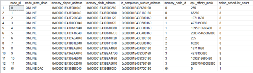
Server MAXDOP is set to 8. In theory, this should be the ideal setup. Microsoft says that they find eight to be the magic number when it comes to scalabilty of parallel processes. If auto soft-NUMA is disabled then there are only four NUMA nodes with one for each memory node. Here’s the output of sys.dm_os_nodes with auto soft-NUMA disabled:

a30_no_auto_soft_numa_dmv

The Test Code

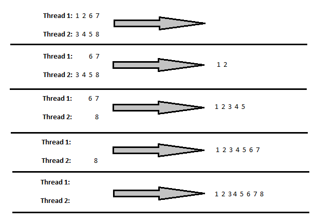
For the test code, I wanted an easy way to alternate sets of parallel queries that finish very quickly with parallel queries that take a long time to finish. I ended up creating a simple stored procedure that only uses the spt_values table and kicks off a user-specified number of parallel queries that finish nearly instanteously followed by a query that cross joins millions of rows together. The final query in the procedure won’t finish in a reasonable amount of time. it is designed to be cancelled. The idea here is to give the observer as much time as needed to poke around various DMVs to make notes about how threads were scheduled.

CREATE OR ALTER PROCEDURE
[dbo].[RUN_SET_OF_QUERIES] (@num_cheap_queries INT) AS
BEGIN
	SET NOCOUNT ON;

	DECLARE @dummy INT,
	@queries_run_so_far INT = 0,
	@filter INT = 0;

	WHILE @queries_run_so_far
		BETWEEN 0 AND @num_cheap_queries - 1
	BEGIN
		SELECT @dummy = MAX(t1.high + t2.high)
		FROM master..spt_values t1
		CROSS JOIN master..spt_values t2
		WHERE @filter = 1
		OPTION (MAXDOP 8);

		SET @queries_run_so_far = @queries_run_so_far + 1;
	END;

	SELECT @dummy =
	MAX(t1.high + t2.high + t3.high + t4.high)
	FROM master..spt_values t1
	CROSS JOIN master..spt_values t2
	CROSS JOIN master..spt_values t3
	CROSS JOIN master..spt_values t4
	OPTION (MAXDOP 8);
END;

To that end, I chose to execute the stored procedure through sqlcmd. The expensive queries don’t modify data so it’s very fast to cancel all of the in-progress queries by closing the sqlcmd window. Readers following along with their 96 core servers at home should feel free to use whatever methodology they wish to kick off the stored procedures. I found it important to be able to kick off the stored procedure with a user-defined time delay between executions and to not have to wait on the completion of the stored procedure before sending more queries. Below is example syntax for a batch file which kicks off four stored procedure calls with a delay of about 2.5 seconds between each call. Each stored procedure executes two fast parallel queries before executing the very expensive one.

 START /B sqlcmd -d {{db_name}} -S {{server_name}} -Q "EXEC [dbo].[RUN_SET_OF_QUERIES] @num_cheap_queries=2" > nul
ping 192.2.0.1 -n 1 -w 2500 > nul
START /B sqlcmd -d {{db_name}} -S {{server_name}} -Q "EXEC [dbo].[RUN_SET_OF_QUERIES] @num_cheap_queries=2" > nul
ping 192.2.0.1 -n 1 -w 2500 > nul
START /B sqlcmd -d {{db_name}} -S {{server_name}} -Q "EXEC [dbo].[RUN_SET_OF_QUERIES] @num_cheap_queries=2" > nul
ping 192.2.0.1 -n 1 -w 2500 > nul
START /B sqlcmd -d {{db_name}} -S {{server_name}} -Q "EXEC [dbo].[RUN_SET_OF_QUERIES] @num_cheap_queries=2" > nul
ping 192.2.0.1 -n 1 -w 2500 > nul

Finally, I needed a query to examine the distribution of parallel workers on the system. In general, you want your parallel workers to be spread out enough so that all schedulers are able to do some useful work. I used the following to get an idea of parallel worker distribution:

SELECT
  session_id
, dop
, start_time
, request_scheduler_id
, STRING_AGG
	(
	CASE WHEN exec_context_id = 0
	THEN NULL ELSE scheduler_id END
	, ','
	)
	WITHIN GROUP (ORDER BY scheduler_id)
	AS used_schedulers_for_parallel_workers
FROM
(
	SELECT
	  dot.session_id
	, dot.scheduler_id
	, dot.exec_context_id
	, req.scheduler_id AS request_scheduler_id
	, req.command
	, req.dop
	, req.start_time
	, dos.parent_node_id
	, dos.cpu_id
	, dos.is_idle
	, dos.load_factor
	, dos.active_workers_count
	FROM
	(
		SELECT DISTINCT
		  session_id
		, scheduler_id
		, exec_context_id
		FROM sys.dm_os_tasks
	) dot
	LEFT OUTER JOIN sys.dm_exec_requests req
		ON dot.session_id = req.session_id
			AND req.request_id = 0
	LEFT OUTER JOIN sys.dm_exec_sessions ses
		ON dot.session_id = ses.session_id
	LEFT OUTER JOIN sys.dm_os_schedulers dos
		ON dos.scheduler_id = dot.scheduler_id
	WHERE ses.is_user_process = 1
) t
GROUP BY
  session_id
, dop
, start_time
, request_scheduler_id
ORDER BY start_time
OPTION (MAXDOP 1);

This query is lazy in that it doesn’t handle plans with multiple parallel zones correctly. However, it works well enough for tests on simple parallel queries (such as the ones for the reproduction forthis post) or for properly written batch mode queries.

Testing with Auto Soft-NUMA

As a reminder, with auto soft-NUMA on my server I had 12 soft-NUMA nodes of 8 schedulers. I restarted SQL Server and ran a .bat file with the following commands repeated 12 times:

START /B sqlcmd -d {{db_name}} -S {{server_name}} -Q "EXEC [dbo].[RUN_SET_OF_QUERIES] @num_cheap_queries=2" > nul
ping 192.2.0.1 -n 1 -w 2500 > nul

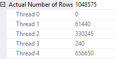
In other words, I kicked off a total of 24 very fast parallel queries and 12 very long running parallel queries. Here is how my scheduling of parallel workers looked:

a30_auto_soft_numa_scheduling

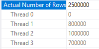
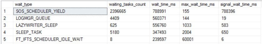
That is a pretty bad outcome. I have 12 MAXDOP 8 queries with all parallel workers assigned to schedulers on just four NUMA nodes. Each CPU in those NUMA nodes has the equivalent of 300% work assigned to it. Execution context 0 doesn’t do much work for the test query, so I have 64 cpus with barely any work to do. It’s unlikely that server CPU will go much higher than 33%. Here are wait stats after running the workload for two minutes:

a30_more_sos_waits

We accumulated two hours of SOS_SCHEDULER_YIELD waits in just two minutes. Not what you want to see with a server that’s around 33% CPU utilization. What went wrong?

Mo’ Schedulers Mo’ Problems

Scheduling of parallel queries was changed in SQL Server 2012. Bob Dorr blogged about it here, and it’s the best source that I’m aware of. Even so, I’ve had a lot of trouble figuring out exactly what the words in that blog post mean. Readers of this blog may be able to relate. I’ve only ever observed the spread selection type in practice, so the most relevant part of the linked post is this one:

Spread: This is the most common decision made by SQL Server. The decision spreads the workers across multiple nodes as required. The design is similar to full except the starting position is based on the saved, next node, global enumerator.

Consider a server with soft-NUMA nodes of 8 schedulers with MAXDOP 8. The first parallel query will be sent to numa node 0. The number of active workers matches the number of schedulers exactly so each active worker is assigned to a different scheduler in the NUMA node. The second parallel query will be sent to NUMA node 1. The third parallel query will be sent to NUMA node 2, and so on. Execution of serial queries or creation of sessions does not matter. That advances a counter that’s separate from the “global enumerator” used for parallel query scheduler placement. As far as I can tell the scheduler assigned to execution context 0 does not affect the scheduling of the parallel worker threads, although it can certainly affect parallel query performance.

The scenario described above doesn’t sound so bad. It can work well if the parallel queries take roughly about the same amount of time to complete and query MAXDOP matches the number of schedulers per soft-NUMA node. Problems can emerge when at least one of those is not true. With the spread selection type it’s possible that the amount of work already assigned to schedulers has no effect on parallel query scheduler placement. Let that sink in. You could have 100 serial queries all assigned to schedulers in numa node 0 but SQL Server may still send a parallel query to that NUMA node. It depends on the position of the “global enumerator” as opposed to current work on the server.

That behavior is why the reproduction in this post works. With a total of 12 soft-NUMA nodes all I need to do is run queries in a fast-fast-slow pattern to cause the slow queries to be doubled and tripled up on schedulers. In some cases sending more parallel queries to a server can be a valid strategy if server CPU isn’t quite as high as you’d like. That might not work here though. Sending more queries will mostly just rack up additional SOS_SCHEDULER_YIELD waits.

It isn’t true that SQL Server never considers the amount of work on a scheduler when assigning parallel worker threads. NUMA nodes have limits on the number of parallel workers as can be seen in sys.dm_exec_query_parallel_workers. There appears to be scheduling choices which consider load factor or worker count when the set of parallel workers only fills part of a soft-NUMA node. Consider a pair of MAXDOP 12 queries running on the same server as described earlier. Suppose that the “global enumerator” starts at position 0. The first query will grab 8 schedulers from NUMA node 0 and 4 schedulers from NUMA node 1. SQL Server has some choice about which schedulers it grabs from NUMA node 1. However, there is no choice to be made for NUMA node 0 because it grabs all of them. The second parallel query grabs 4 schedulers from NUMA node 1 and 8 schedulers from NUMA node 2. Again, SQL server can make a choice about which schedulers it uses from NUMA node 1. That decision can factor in system load. Just like with serial queries, if queries are sent too quickly to the server then you might see unnecessary doubling up of schedulers in NUMA node 1.

I didn’t try to dig into the details fully, but hopefully the above gives you a high level understanding of what kind of problems you might see with parallel query scheduling on servers with more than one NUMA node.

Testing Without Auto Soft-NUMA

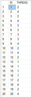
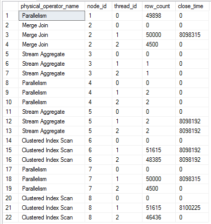
Armed with our new knowledge, let’s consider what might happen with the previous workload if auto soft-NUMA is disabled. Assume that the server was restarted and the global enumerator starts at position 0. Three MAXDOP 8 queries are able to fit into each NUMA node of 24 schedulers. The expensive query for the first execution of the stored procedure will be sent to schedulers on the first NUMA node. The expensive query for the second execution of the stored procedure will be sent to schedulers on the second NUMA node, the third will be sent to the third NUMA node, and the fourth will be sent to the fourth NUMA node. As we continue to execute more queries we’ll loop around but the key difference is that SQL Server is able to place the parallel worker threads however it wants on the 24 schedulers. It can look at things like load factor or the number of workers per scheduler. After all 12 stored procedures have started we can end up with scheduling like this:

a30_good_scheduling

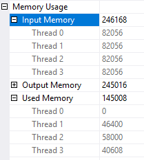
Every scheduler has at least one thread for a parallel worker or an execution context 0 thread. Scheduler 22 is one of eight schedulers with more than one parallel worker assigned. Execution context 0 for these queries is expected to do very little work, so it could be argued that a better distribution would be to have exactly one parallel worker per scheduler. However, overall this is a pretty good distribution and we can push server CPU to 90%. After two minutes of execution we have significantly fewer time spent on SOS_SCHEDULER_YIELD waits compared to before:

a30_less_sos_waits

In this situation, we can see a significant improvement in server resource utilization by disabling auto soft-NUMA. For other workloads and query mixes the scheduling behavior offered with auto soft-NUMA may be a better fit. Key factors include the patttern of parallel queries, MAXDOP, and the number of schedulers per memory node.

Final Thoughts

We observed a bottleneck with SOS_SCHEDULER_YIELD waits for an ETL workload for which it was not easy to scale up the number of queries. This can happen if there are only so many partitions to process or if ETL queries require large memory grants, say, for compressing columnstore data. We were able to shave 30% off the overall workload time by using Resource Governor CPU affinity and doing our own scheduling. Less drastic workarounds include disabling auto soft-NUMA, changing MAXDOP, increasing CTFP, or reigning in some queries which don’t need to run in parallel. Thanks for reading!

Advertisement

The Return of RESERVED_MEMORY_ALLOCATION_EXT

It is possible to see a scalability bottleneck in the form of high average wait time for the RESERVED_MEMORY_ALLOCATION_EXT wait if a highly concurrent workload is run on a server that consumes memory with batch mode operators. I believe that the severity of the bottleneck depends on unknown factors in the server’s initial memory state and the rate of memory actually used by queries to run batch mode operations. This blog post shares a reproduction of the issue along with a call to action.

The Test Query

Data prep for the test query is very simple. We throw the first ten million sequential integers into two single column BIGINT tables. Additionally, an empty CCI is created to add eligibility for batch mode as desired:

DROP TABLE IF EXISTS DUMMY_CCI;
CREATE TABLE DUMMY_CCI (
	ID INT,
	INDEX CCI CLUSTERED COLUMNSTORE
);

DROP TABLE IF EXISTS HASH_JOIN_SCALE_TEST_1;
CREATE TABLE HASH_JOIN_SCALE_TEST_1 (
	ID BIGINT NOT NULL
);

INSERT INTO HASH_JOIN_SCALE_TEST_1 WITH (TABLOCK)
SELECT TOP (10000000) ROW_NUMBER()
	OVER (ORDER BY (SELECT NULL))
FROM master..spt_values t1
CROSS JOIN master..spt_values t2
CROSS JOIN master..spt_values t3
OPTION (MAXDOP 1);

DROP TABLE IF EXISTS HASH_JOIN_SCALE_TEST_2;
CREATE TABLE HASH_JOIN_SCALE_TEST_2 (
ID BIGINT NOT NULL
);

INSERT INTO HASH_JOIN_SCALE_TEST_2 WITH (TABLOCK)
SELECT TOP (10000000) ROW_NUMBER()
	OVER (ORDER BY (SELECT NULL))
FROM master..spt_values t1
CROSS JOIN master..spt_values t2
CROSS JOIN master..spt_values t3
OPTION (MAXDOP 1);

The SELECT query that we’re going to test with joins them together and returns a count of distinct IDs:

SELECT COUNT(DISTINCT t1.ID)
FROM dbo.HASH_JOIN_SCALE_TEST_1 t1
LEFT OUTER JOIN dbo.HASH_JOIN_SCALE_TEST_2 t2
	ON t1.ID = t2.ID
OPTION (MAXDOP 1);

This is certainly an odd thing to do, but the point of this query is to create a simple test case that uses a bit of memory to create hash tables. Without any indexes on the table we’re very likely to get a hash join. In row mode the query takes about 17 seconds on the test server and uses 1257528 KB of memory.

As far as I can tell this query is a good fit for batch mode. The join is on BIGINT columns and everything except for the rowstore scans can execute in batch mode:

a28_query_plan

Even with the hidden conversions of 20 million rows from row mode to batch mode the query finishes in about 5 seconds. It uses significantly less memory compared to the row mode query: 386112 KB. All of this seems very reasonable.

Testing at Scale

The situation becomes less reasonable once there are many concurrent queries running at once. We go from the batch mode query running in a third of the time of row mode to sometimes running slower. Testing was done with 96 concurrent queries each running queries until 576 total queries were completed. Below is a graph of OS CPU and OS privileged time CPU based on perfmon data:

a28_cpu_graphs

The first third of the graph corresponds to the batch mode workload. CPU never hits 100% and is extremely variable during the run. We also see a high amount of privileged time in the OS. Within SQL Server, we use a total of 222,400,512 KB of query memory. The total wait time for RESERVED_MEMORY_ALLOCATION_EXT can vary, but for this one it was around 11.5 million ms.

The second third of the graph is the part that resets the server memory state. As stated in the introduction, this scalability bottleneck doesn’t always happen and seems to have some kind of dependency on the server’s initial memory state. Here we do a SELECT COUNT(*) on a 1 TB table to add pressure to the rowstore buffer pool.

The final third of the graph corresponds to the row mode workload. CPU jumps to near 100% very quickly and doesn’t waver much during the run. There is very little privileged time in the OS. Within SQL Server, we use a total of 724,336,128 KB of query memory. The wait time for RESERVED_MEMORY_ALLOCATION_EXT is always significantly reduced compared to batch mode. For this run it was around 107k ms.

In conclusion, we see about 1% of memory wait time with the row mode workload compared to the batch mode workload. Usually the row mode workload finishes a little faster than the batch mode one, despite needing over 3X as much total memory and the per-query efficiency advantage of batch mode.

Speculation on the Problem

There may be a hint in the memory management architecture guide:

Starting with SQL Server 2012, SQL Server might allocate more memory than the value specified in the max server memory setting. This behavior may occur when the Total Server Memory (KB) value has already reached the Target Server Memory (KB) setting (as specified by max server memory). If there is insufficient contiguous free memory to meet the demand of multi-page memory requests (more than 8 KB) because of memory fragmentation, SQL Server can perform over-commitment instead of rejecting the memory request.

This behavior is typically observed during the following operations: Large Columnstore index queries.

There are observable differences in how memory is allocated for the same operator when switching from batch mode to row mode. The number of wait events for RESERVED_MEMORY_ALLOCATION_EXT is significantly higher for row mode compared to batch mode. In addition, it remains nearly constant when TF 834 is enabled:

a28_memory_waits

TF 834 appears to fully resolve the scalability issue with batch mode, just like last time. It offers a dramatic improvement in workload completion time:

a28_summary_of_timings

Perhaps some batch mode operators require contiguous free memory for their allocations but the same operation done through row mode does not have that restriction. I can’t go any further than this because I don’t know anything about OS internals or memory management, but it could explain why we see such different behavior between row mode and batch mode.

Use Your Voice

Since SQL Server 2012, Microsoft has listed TF 834 as incompatible with columnstore. There are lots of scary consequences:

  • A non-yielding scheduler error and associated memory dumps in the SQL Server Error log.
  • Columnstore queries trigger severe performance issues.
  • A SQL Server instance triggers access violations when you execute Columnstore queries.
  • You encounter the following error when you run sp_createstats

However, I’ve been told that many of the SQL Server columnstore benchmarks for the TPC-H benchmarks use TF 834. It seems to be a natural fit for columnstore, and there are some workloads (seen in the lab and reproduced in the last two blog posts) where it resolves a key scalability bottleneck which is difficult to address through other means. I have created a feedback item on UserVoice requesting that Microsoft support TF 834 with columnstore.

Final Thoughts

Please provide feedback on the UserVoice item if you are able to do so. Thanks for reading!

Large CCI ETLs Cannot Scale Without TF 834

Large servers may experience a scalability bottleneck related to the RESERVED_MEMORY_ALLOCATION_EXT wait event during loading of columnstore tables. This blog post shares a reproduction of the issue and discusses some test results.

The Test Server

Testing was done on a four socket bare metal server with 24 cores per socket. The server had 1 TB of RAM and storage was provided by a SAN. Within SQL Server, we were able to read data at a peak rate of about 5.5 GB/s. Hyperthreading was disabled, but there aren’t any other nonstandard OS configuration settings that I’m aware of.

SQL Server 2016 SP1 CU7 was installed on Windows Server 2016. Most default settings were retained for this testing, including allowing auto soft-NUMA to break up the 96 schedulers into 12 groups of 8, with 3 per memory node. Max server memory was set to around 800000 MB. The user database had 24 data files, indirect checkpoints weren’t used, and the memory model in use was conventional. No interesting trace flags were enabled, except perhaps for TF 4199. I did grow max server memory to close to the maximum before starting any of the tests.

Testing Code and Method

The workload test loaded the same data from a SQL Server table into 576 CCI target tables. For my testing I used a source table of one million rows. Each session grabs a number from a sequence, loads data into the table corresponding to the sequence number, and continues to do that until there are no more tables to process. This may seem like an odd test to run, but think of it as an abstract representation of a columnstore ETL workload which loads data into partitioned CCIs.

The first step is to define the source table. I created a 50 column table that stored only 0s in all of its rows. There’s nothing particularly special about this choice other that it has a very low disk footprint as a CCI because it compresses so well. On a non-busy system it took around 7.3 seconds to insert one million rows into a CCI. Below is the table definition:

DROP TABLE IF EXISTS CCI_SOURCE;

CREATE TABLE CCI_SOURCE (
ID1 SMALLINT,
ID2 SMALLINT,
ID3 SMALLINT,
ID4 SMALLINT,
ID5 SMALLINT,
ID6 SMALLINT,
ID7 SMALLINT,
ID8 SMALLINT,
ID9 SMALLINT,
ID10 SMALLINT,
ID11 SMALLINT,
ID12 SMALLINT,
ID13 SMALLINT,
ID14 SMALLINT,
ID15 SMALLINT,
ID16 SMALLINT,
ID17 SMALLINT,
ID18 SMALLINT,
ID19 SMALLINT,
ID20 SMALLINT,
ID21 SMALLINT,
ID22 SMALLINT,
ID23 SMALLINT,
ID24 SMALLINT,
ID25 SMALLINT,
ID26 SMALLINT,
ID27 SMALLINT,
ID28 SMALLINT,
ID29 SMALLINT,
ID30 SMALLINT,
ID31 SMALLINT,
ID32 SMALLINT,
ID33 SMALLINT,
ID34 SMALLINT,
ID35 SMALLINT,
ID36 SMALLINT,
ID37 SMALLINT,
ID38 SMALLINT,
ID39 SMALLINT,
ID40 SMALLINT,
ID41 SMALLINT,
ID42 SMALLINT,
ID43 SMALLINT,
ID44 SMALLINT,
ID45 SMALLINT,
ID46 SMALLINT,
ID47 SMALLINT,
ID48 SMALLINT,
ID49 SMALLINT,
ID50 SMALLINT
);

INSERT INTO CCI_SOURCE WITH (TABLOCK)
SELECT
 ID,ID,ID,ID,ID,ID,ID,ID,ID,ID
,ID,ID,ID,ID,ID,ID,ID,ID,ID,ID
FROM (
	SELECT TOP (1000000) 0 ID
	FROM master..spt_values t1
	CROSS JOIN master..spt_values t2
) t;

Next we need a stored procedure that can save off previous test results (as desired) and reset the server for the next test. If a test name is passed in then results are saved to CCI_TEST_RESULTS and CCI_TEST_WAIT_STATS from the previous run. The procedure always recreates all of the target CCI tables, resets the sequence, clears the buffer pool, and does a few other things.

CREATE OR ALTER PROCEDURE [dbo].[CCI_TEST_RESET] (@PreviousTestName NVARCHAR(100) = NULL, @DebugMe INT = 0)
AS
BEGIN
	DECLARE
	@tablename SYSNAME,
	@table_number INT = 1,
	@SQLToExecute NVARCHAR(4000);

	/*
CREATE TABLE CCI_TEST_WAIT_STATS (
	TEST_NAME NVARCHAR(100),
	WAIT_TYPE NVARCHAR(60),
	WAITING_TASKS_COUNT BIGINT,
	WAIT_TIME_MS BIGINT,
	MAX_WAIT_TIME_MS BIGINT,
	SIGNAL_WAIT_TIME_MS BIGINT
);

CREATE TABLE CCI_TEST_RESULTS (
	TEST_NAME NVARCHAR(100),
	TOTAL_SESSION_COUNT SMALLINT,
	TEST_DURATION INT,
	TOTAL_WORK_TIME INT,
	BEST_TABLE_TIME INT,
	WORST_TABLE_TIME INT,
	TOTAL_TABLES_PROCESSED SMALLINT,
	MIN_TABLES_PROCESSED SMALLINT,
	MAX_TABLES_PROCESSED SMALLINT
);
	*/

	SET NOCOUNT ON;

	IF @DebugMe = 0
	BEGIN
		DROP SEQUENCE IF EXISTS CCI_PARALLEL_TEST_SEQ;
		CREATE SEQUENCE CCI_PARALLEL_TEST_SEQ
			AS SMALLINT
			START WITH 1
			INCREMENT BY 1
			CACHE 600;

		IF @PreviousTestName  N''
		BEGIN
			INSERT INTO CCI_TEST_RESULTS WITH (TABLOCK)
			SELECT @PreviousTestName,
			  COUNT(*) TOTAL_SESSION_COUNT
			, DATEDIFF(MILLISECOND, MIN(MIN_START_TIME), MAX(MAX_END_TIME)) TEST_DURATION
			, SUM(TOTAL_SESSION_TIME) TOTAL_WORK_TIME
			, MIN(MIN_TABLE_TIME) BEST_TABLE_TIME
			, MAX(MAX_TABLE_TABLE) WORST_TABLE_TIME
			, SUM(CNT) TOTAL_TABLES_PROCESSED
			, MIN(CNT) MIN_TABLES_PROCESSED
			, MAX(CNT) MAX_TABLES_PROCESSED
			FROM (
				SELECT
				  SESSION_ID
				, COUNT(*) CNT
				, SUM(DATEDIFF(MILLISECOND, START_TIME, END_TIME)) TOTAL_SESSION_TIME
				, MIN(DATEDIFF(MILLISECOND, START_TIME, END_TIME)) MIN_TABLE_TIME
				, MAX(DATEDIFF(MILLISECOND, START_TIME, END_TIME)) MAX_TABLE_TABLE
				, MIN(START_TIME) MIN_START_TIME
				, MAX(END_TIME) MAX_END_TIME
				FROM CCI_TEST_LOGGING_TABLE
				GROUP BY SESSION_ID
			) t;

			INSERT INTO CCI_TEST_WAIT_STATS WITH (TABLOCK)
			SELECT @PreviousTestName, * FROM sys.dm_os_wait_stats
			WHERE wait_type IN (
				'RESERVED_MEMORY_ALLOCATION_EXT'
				, 'SOS_SCHEDULER_YIELD'
				, 'PAGEIOLATCH_EX'
				, 'MEMORY_ALLOCATION_EXT'
				, 'PAGELATCH_UP'
				, 'PAGEIOLATCH_SH'
				, 'WRITELOG'
				, 'LATCH_EX'
				, 'PAGELATCH_EX'
				, 'PAGELATCH_SH'
				, 'CMEMTHREAD'
				, 'LATCH_SH'
			);

		END;

		DROP TABLE IF EXISTS CCI_TEST_LOGGING_TABLE;
		CREATE TABLE CCI_TEST_LOGGING_TABLE (
			SESSION_ID INT,
			TABLE_NUMBER INT,
			START_TIME DATETIME,
			END_TIME DATETIME
		);

	END;

	WHILE @table_number BETWEEN 0 AND 576
	BEGIN
		SET @tablename = N'CCI_PARALLEL_RPT_TARGET_' + CAST(@table_number AS NVARCHAR(3));
		SET @SQLToExecute= N'DROP TABLE IF EXISTS ' + QUOTENAME(@tablename);
		IF @DebugMe = 1
		BEGIN
			PRINT @SQLToExecute;
		END
		ELSE
		BEGIN
			EXEC (@SQLToExecute);
		END;

		SET @SQLToExecute = N'SELECT * INTO ' + QUOTENAME(@tablename) +
		' FROM CCI_SOURCE WHERE 1 = 0';
		IF @DebugMe = 1
		BEGIN
			PRINT @SQLToExecute;
		END
		ELSE
		BEGIN
			EXEC (@SQLToExecute);
		END;

		SET @SQLToExecute = N'CREATE CLUSTERED COLUMNSTORE INDEX CCI ON ' + QUOTENAME(@tablename);
		IF @DebugMe = 1
		BEGIN
			PRINT @SQLToExecute;
		END
		ELSE
		BEGIN
			EXEC (@SQLToExecute);
		END;

		SET @table_number = @table_number + 1;
	END;

	IF @DebugMe = 0
	BEGIN
		DBCC DROPCLEANBUFFERS WITH NO_INFOMSGS;
		DBCC FREEPROCCACHE WITH NO_INFOMSGS;
		DBCC FREESYSTEMCACHE('ALL');

		SELECT COUNT(*) FROM CCI_SOURCE; -- read into cache

		DBCC SQLPERF ("sys.dm_os_wait_stats", CLEAR) WITH NO_INFOMSGS;
		DBCC SQLPERF ("sys.dm_os_spinlock_stats", CLEAR) WITH NO_INFOMSGS;
	END;
END;

Finally we need a stored procedure that can be called to do as many CCI inserts as it can as quickly as possible. I used the following code:

CREATE OR ALTER PROCEDURE [dbo].[CCI_RUN_INSERTS] (@DebugMe INT = 0)
AS
BEGIN
	DECLARE @table_number INT,
	@tablename SYSNAME,
	@SQLToExecute NVARCHAR(4000),
	@start_loop_time DATETIME;

	SET NOCOUNT ON;

	SELECT @table_number = NEXT VALUE FOR CCI_PARALLEL_TEST_SEQ;

	WHILE @table_number BETWEEN 0 AND 576
	BEGIN
		SET @start_loop_time = GETDATE();

		SET @tablename = N'CCI_PARALLEL_RPT_TARGET_' + CAST(@table_number AS NVARCHAR(3));
		SET @SQLToExecute= N'
		INSERT INTO ' + QUOTENAME(@tablename) + N' WITH (TABLOCK)
		SELECT * FROM CCI_SOURCE WITH (TABLOCK)
		OPTION (MAXDOP 1)';

		IF @DebugMe = 1
		BEGIN
			PRINT @SQLToExecute;
		END
		ELSE
		BEGIN
			EXEC (@SQLToExecute);

			INSERT INTO CCI_TEST_LOGGING_TABLE VALUES (@@SPID, @table_number, @start_loop_time, GETDATE());
		END;

		SELECT @table_number = NEXT VALUE FOR CCI_PARALLEL_TEST_SEQ;
	END;
END;

To vary the number of concurrent queries I used sqlcmd. Each set of 12 sessions had the following format:

START /B sqlcmd -d your_db_name -S your_server_name -Q "EXEC dbo.[CCI_RUN_INSERTS]" > nul
ping 192.2.0.1 -n 1 -w 1 > nul

My workflow was to perform this test was to add the desired number of calls to the stored procedure in the .bat file, run the test, and to check the results to make sure that the test was a good one. If it was I saved off results using the reset procedure. If not I ran the reset procedure and tried again.

The ping command is there to add a small delay between sets of queries. I found that adding such a delay led to less doubling up on schedulers. I picked 12 because that’s the number of soft-NUMA nodes. Sometimes tests would get quite a bit of SOS_SCHEDULER_YIELD waits which would mean that they couldn’t be accurately compared to other tests. My fix was to just run the test again. It required a bit of patience but I never had to run a test more than once. SOS waits weren’t eliminated but I’d say they fell to acceptable levels:

a27_SOS_CPU_wait_table

The right way to avoid SOS waits for testing like this (which might require every user session to go on its own scheduler) would be to set up 96 manual soft-NUMA nodes. But who has time for that?

Test Results

12 tests with different numbers of active queries were run. I picked numbers that somewhat evenly divided into 576 to try to keep work balanced between threads. The blue line in the chart below measures how long each test took from start to finish and the orange line represents how fast the test could have completed if there was no contention on the server whatsoever:

a27_No_T834_compare_chart

Naturally we can’t expect the two lines to match perfectly, but improvements in runtime stop after going past 32 threads. In fact, the workload takes longer with 96 threads compared to 32 threads.

The dominant wait event for the higher thread count runs is RESERVED_MEMORY_ALLOCATION_EXT. Below is a chart of all of the wait events worth mentioning for the 96 thread run:

a27_no_T834_wait_table

The total number of wait events for RESERVED_MEMORY_ALLOCATION_EXT is very consistent between runs. However, the average wait time significantly increases as the number of concurrent queries increases:

a27_memory_waits_chart

In fact, it could be said that that nearly all worker time past 32 threads is spent waiting on memory. The final column in the chart below is the total time spent in SQL Server minus wait time for RESERVED_MEMORY_ALLOCATION_EXT. The values in that column are remarkably consistent.

a27_No_TF_834_summary

In my experience, when we get into a situation with high memory waits caused by too much concurrent CCI activity all queries on the server that use a memory grant can be affected. For example, I’ve seen sp_whoisactive run for longer than 90 seconds.

It needs to be stated that not all CCIs will suffer from this scalability problem. I was able to achieve good scalability with some artificial tables, but all of the real target tables that I tested have excessive memory waits at high concurrency. Perhaps tables which require more CPU to compress naturally spread out their memory requests and the underlying OS is better able to keep up.

Test Results With Trace Flag 834

Microsoft strongly recommends against using trace flag 834 with columnstore tables. There’s even an article dedicated to that warning. I was desperate so I tried it anyway. The difference was night and day:

a27_T834_compare_chart

Enabling trace flag 834 does at least three things: SQL Server grows to max server memory on startup, AWE memory is used for memory access, and large pages are used for the buffer pool. I didn’t see gains when using LPIM (which uses AWE memory) or by growing memory to max before running tests with a conventional memory model, so I suspect that the large pages are making a key difference. Wait time for RESERVED_MEMORY_ALLOCATION_EXT is under a second for all tests.

Scalability is diminished a bit for the 96 thread run. There are some wait events that creep up:

TF_834_96_thread_wait_stats

All of the wait events can be troubleshooted in conventional ways except possibly for CMEMTHREAD. There’s no longer a large amount of time spent outside of SQL Server in the OS.

Other Workarounds

Without trace flag 834 this can be a difficult problem to work around. The two main strategies are to spread out CCI insert activity as much as possible during the ETL and to reduce memory usage of queries which run at the same time as the CCI inserts. For example, consider a query that inserts into a CCI that also performs a large hash join. If that hash join can be moved to somewhere else in the process then you might come out ahead in reducing contention on memory.

Other than that, there’s some evidence that virtualized servers are not a good fit for this type of workload. Large virtual guests experience the memory waits at an increased rate, but it isn’t yet clear if the problem can be avoided through some change in VM configuration.

Final Thoughts

It’s hard not to conclude that TF 834 is necessary to get scalability for columnstore ETLs on very large servers. Hopefully Microsoft will make TF 834 compatible with columnstore one day in the future. Thanks for reading!

Batch Mode Memory Fractions

My least favorite tempdb spills are the ones that happen with a large percentage of the memory grant remaining unused. For example, recently I saw tempdb spills with a memory grant of 35 GB but SQL Server reported that only 10 GB of memory was used. Usually this problem can be traced back to suboptimal memory fractions somewhere in a query plan. I suspect that it can also happen with certain types of queries that load data into columnstore tables but haven’t verified that. In the test environment the issue was caused by memory fractions, but these memory fractions were attached to batch mode operators. The rules for batch mode memory fractions certainly appear to be different than those for rowstore memory fractions. I believe that I was able to work out a few of the details for a few simple cases. In some scenarios, plans with multiple batch mode hash joins can ask for significantly more memory than needed. Reducing the memory grant via Resource Governor or a query hint to something more reasonable can lead to unnecessary (and often frustrating) tempdb spills.

What is a Memory Fraction?

There’s very little information out there about memory fractions. I would define them as information in the query plan that can give you clues about each operator’s share of the total query memory grant. This is naturally more complicated for query plans that insert into tables with columnstore indexes but that won’t be covered here. Most references will tell you not to worry about memory fractions or that they aren’t useful most of the time. Out of thousands of queries that I’ve tuned I can only think of a few for which memory fractions were relevant. Sometimes queries spill to tempdb even though SQL Server reports that a lot of query memory was unused. In these situations I generally hope for a poor cardinality estimate which leads to a memory fraction which is too low for the spilling operator. If fixing the cardinality estimate doesn’t prevent the spill then things can get a lot more complicated, assuming that you don’t just give up.

Types of Query Plans

The demos for this blog post all use tables with identical structures and data. The tables are heaps so the plans will only feature hash joins. The most important plan characteristic is how many of the hash tables need to be kept in memory concurrently while the query processor executes the query. This is where memory fractions come in. The query optimizer tries to reuse parts of memory grants as it can. For example, if the hash build for the first join isn’t needed when the third join executes then it’s possible to use the memory grant from the first hash table for the third hash table. Some of the examples below will make this more clear.

The first type of plan has hash joins which can all run concurrently. Memory for the hash tables cannot be reused between operators.

a26_concurrent_joins

For that query, the MF_DEMO_1 table is the probe side for all of the joins. SQL Server builds all of the hash joins and then rows flow from the probe side through the plan (as long as there aren’t tempdb spills). I will refer to this type of plan as a “concurrent join plan” which is a term that I just made up.

The second type of plan has hash joins which cannot all run concurrently. Pairs of hash tables are active at the same time, but memory grants can be reused between operators.

s26_nonconcurrent_joins

For that query, the MF_DEMO_1 table is the build side for all of the joins. Each hash table blocks the next one from starting. This means that at most two hash tables need to be kept in memory at the same time. Query memory cannot be reused for joins 1 and 2 but join 3 can reuse memory from join 1 and join 4 can reuse memory from join 2. I will refer to this type of plan as a “nonconcurrent join plan” which is another term that I just made up.

If the above wasn’t clear I recommend running through the demos with live query statistics enabled. It can be very useful to understand how rows flow through a plan. As far as I know, all queries of this type can be implemented with the nonconcurrent pattern but not all queries can be implemented with the concurrent pattern .

Create the Tables

The table definitions for our demos are pretty boring. I’m using a VARCHAR(100) as the join column to blow up memory grants and requirements a bit. All of the tables are heaps and have about 6.5 million rows in them. TARGET_TABLE is used as a dumping ground for the inserts and #ADD_BATCH_MODE is used to switch the hash joins to batch mode as desired. All testing was done on SQL Server 2016 SP1 CU7.

DROP TABLE IF EXISTS MF_DEMO_1;
CREATE TABLE MF_DEMO_1 (
       ID VARCHAR(100)
);

INSERT INTO MF_DEMO_1 WITH (TABLOCK)
SELECT 999999999999999 + ROW_NUMBER()
	OVER (ORDER BY (SELECT NULL))
FROM master..spt_values t1
CROSS JOIN master..spt_values t2;

CREATE STATISTICS S1 ON MF_DEMO_1 (ID) WITH FULLSCAN;

DROP TABLE IF EXISTS MF_DEMO_2;
CREATE TABLE MF_DEMO_2 (
       ID VARCHAR(100)
);

INSERT INTO MF_DEMO_2 WITH (TABLOCK)
SELECT 999999999999999 + ROW_NUMBER()
	OVER (ORDER BY (SELECT NULL))
FROM master..spt_values t1
CROSS JOIN master..spt_values t2;

CREATE STATISTICS S2 ON MF_DEMO_2 (ID) WITH FULLSCAN;

DROP TABLE IF EXISTS MF_DEMO_3;
CREATE TABLE MF_DEMO_3 (
       ID VARCHAR(100)
); 

INSERT INTO MF_DEMO_3 WITH (TABLOCK)
SELECT 999999999999999 + ROW_NUMBER()
	OVER (ORDER BY (SELECT NULL))
FROM master..spt_values t1
CROSS JOIN master..spt_values t2;

CREATE STATISTICS S3 ON MF_DEMO_3 (ID) WITH FULLSCAN;

DROP TABLE IF EXISTS MF_DEMO_4;
CREATE TABLE MF_DEMO_4 (
       ID VARCHAR(100)
); 

INSERT INTO MF_DEMO_4 WITH (TABLOCK)
SELECT 999999999999999 + ROW_NUMBER()
	OVER (ORDER BY (SELECT NULL))
FROM master..spt_values t1
CROSS JOIN master..spt_values t2;

CREATE STATISTICS S4 ON MF_DEMO_4 (ID) WITH FULLSCAN;

DROP TABLE IF EXISTS MF_DEMO_5;
CREATE TABLE MF_DEMO_5 (
	ID VARCHAR(100)
); 

INSERT INTO MF_DEMO_5 WITH (TABLOCK)
SELECT 999999999999999 + ROW_NUMBER()
	OVER (ORDER BY (SELECT NULL))
FROM master..spt_values t1
CROSS JOIN master..spt_values t2;

CREATE STATISTICS S5 ON MF_DEMO_5 (ID) WITH FULLSCAN;

CREATE TABLE #ADD_BATCH_MODE (I INT, INDEX CCI CLUSTERED COLUMNSTORE);

DROP TABLE IF EXISTS TARGET_TABLE;

CREATE TABLE TARGET_TABLE (ID VARCHAR(100));

Row Mode Memory Fractions For Concurrent Join Plans

The following query results in a concurrent join plan with row mode hash joins:

INSERT INTO TARGET_TABLE WITH (TABLOCK)
SELECT t1.ID
FROM MF_DEMO_3 t3
RIGHT OUTER JOIN MF_DEMO_2 t2
RIGHT OUTER JOIN MF_DEMO_1 t1
ON t1.ID = t2.ID
ON t1.ID = t3.ID
OPTION (FORCE ORDER, MAXDOP 1);

The desired memory grant is 2860640 KB. The memory fractions for both join operators have an input of 0.5 and an output of 0.5. This is exactly as expected. The hash tables can both start at the same time and cannot reuse memory, so each operator gets 50% of the query memory grant for the plan. Adding a third join to the plan increases the query memory grant to 4290960 KB.

INSERT INTO TARGET_TABLE WITH (TABLOCK)
SELECT t1.ID
FROM MF_DEMO_4 t4
RIGHT OUTER JOIN MF_DEMO_3 t3
RIGHT OUTER JOIN MF_DEMO_2 t2
RIGHT OUTER JOIN MF_DEMO_1 t1
ON t1.ID = t2.ID
ON t1.ID = t3.ID
ON t1.ID = t4.ID
OPTION (FORCE ORDER, MAXDOP 1);

Again, this seems very reasonable. SQL Server now tries to builds three hash tables in memory at the same time. The memory fractions for each operator have fallen to 0.3333333. Each operator gets a third of the query memory grant.

Row Mode Memory Fractions For Nonconcurrent Join Plans

The following query results in a nonconcurrent join plan with row mode hash joins:

INSERT INTO TARGET_TABLE WITH (TABLOCK)
SELECT t1.ID
FROM MF_DEMO_1 t1
INNER JOIN MF_DEMO_2 t2 ON t1.ID = t2.ID
INNER JOIN MF_DEMO_3 t3 ON t2.ID = t3.ID
INNER JOIN MF_DEMO_4 t4 ON t3.ID = t4.ID
OPTION (MAXDOP 1, FORCE ORDER);

The query plan was uploaded here. I recommend downloading the all of the plans referenced in this blost post if you’re interested in them so you can see all of the details.

Here are the memory fractions for the rightmost join (node 3):

Memory Fractions Input: 1, Memory Fractions Output: 0.476174

here are the memory fractions for the middle join (node 2):

Memory Fractions Input: 0.523826, Memory Fractions Output: 0.5

and here are the memory fractions for the leftmost join (node 1):

Memory Fractions Input: 0.5, Memory Fractions Output: 1

What do all of those numbers mean? The rightmost join builds its hash table first and starts with all query memory available to it. However, the output fraction is 0.476174. That means that the hash table can only use up to 47.6% of the query memory granted to the plan. The middle join is able to use up to 50% (the minimum of the input and output fractions for the node) of the memory granted to the plan. Note that 0.476174 + 0.523826 = 1.0. The last join to start executing is also able to use up to 50% of the granted memory. That join is the last operator that uses memory in the plan so the output fraction is 1.0. Memory grant reuse allows the plan to use up to 147.6% of the memory grant over the lifetime of the query execution. Without memory grant reuse each operator wouldn’t be able to use as much memory.

Removing one of the joins results in the desired query memory grant dropping from 3146704 KB to 3003672 KB. This is a significantly less drop than the other query. The smaller decrease is expected because the third join that we added can reuse the memory grant from the first. As more joins are added to a nonconcurrent plan the desired memory grant grows at a much slower rate than the memory grant for the concurrent join plan.

Batch Mode Memory Fractions For Concurrent Join Plans

The query plan for the next query is somewhat dependent on hardware. On my machine I had to let it run in parallel to get batch mode hash joins:

INSERT INTO TARGET_TABLE WITH (TABLOCK)
SELECT t1.ID
FROM MF_DEMO_5 t5
RIGHT OUTER JOIN MF_DEMO_4 t4
RIGHT OUTER JOIN MF_DEMO_3 t3
RIGHT OUTER JOIN MF_DEMO_2 t2
RIGHT OUTER JOIN MF_DEMO_1 t1
LEFT OUTER JOIN #ADD_BATCH_MODE ON 1 = 0
ON t1.ID = t2.ID
ON t1.ID = t3.ID
ON t1.ID = t4.ID
ON t1.ID = t5.ID
OPTION (FORCE ORDER, MAXDOP 4);

The estimated plan is here. It’s easy to tell if the query is using batch mode joins because the joins are run in parallel but there are no repartition stream operators.

a26_concurrent_joins_batch

SQL Server is not able to reuse memory grants for this query. SQL Server tries to build all of the hash tables in memory before probe side is processed. However, the memory fractions are different from before: 0.25, 0.5, 0.75, and 1.0. These memory fractions do not make sense if interpreted in the same way as before. How can the final hash join in the plan have an input memory fraction of 1.0?

It’s unclear what the memory fractions are supposed to mean here, but there is one observable difference compared to the row mode plan. In the row mode equivalent plan SQL Server divides the memory evenly between operators. For our very simple test plan this means that all of the hash joins will spill to tempdb or none of them will spill. Reducing a MAX_GRANT_PERCENT hint from the right value by 1% results in two spills:

a26_row_mode_spill

Both operators spilled because memory was divided evenly and there wasn’t enough memory to hold both hash tables in memory. However, with batch mode hash joins we can get plans like the following:

a26_batch_spill

How is it possible that one join spills but the other doesn’t? It is only possible if memory isn’t divided evenly. It appears that memory is used as needed in some situations. Unfortunately, the actual plan for batch mode operators doesn’t give us a lot of spill information like it does for row mode. There’s a debug channel extended event query_execution_batch_hash_join_spilled that can give us some clues. 657920 KB of memory was granted for a two batch mode hash join query. For the operator that spilled, only 44852457 bytes were written to memory on the build side. That’s about 43800 KB, which is significantly less than half of available query memory.

a26_concurrent_spill_XE

We can’t conclude that exactly 44852457 bytes of memory were granted to the operator. However, it should be somewhat close. In conclusion, for these types of queries it isn’t clear what the memory grant fractions are supposed to mean. SQL Server is able to exceed them in some cases. It’s possible to see 0 bytes of memory used for the build side in the extended event. I believe that this is the bad type of memory reuse as opposed to the good kind.

Batch Mode Memory Fractions For Nonconcurrent Join Plans

The following query results in a nonconcurrent batch mode hash join plan on my machine:

INSERT INTO TARGET_TABLE WITH (TABLOCK)
SELECT t1.ID
FROM MF_DEMO_1 t1
LEFT OUTER JOIN #ADD_BATCH_MODE On 1 = 0
WHERE EXISTS (
	SELECT 1
	FROM MF_DEMO_2 t2 WHERE t1.ID = t2.ID
) AND EXISTS (
	SELECT 1
	FROM MF_DEMO_3 t3 WHERE t1.ID = t3.ID
) AND EXISTS (
	SELECT 1
	FROM MF_DEMO_4 t4 WHERE t1.ID = t4.ID
) AND EXISTS (
	SELECT 1
	FROM MF_DEMO_5 t5 WHERE t1.ID = t5.ID
) OPTION (MAXDOP 4, FORCE ORDER);

As far as I know there’s nothing special about the semijoins. I used them to keep the estimated row size as consistent as possible. The behavior detailed below can be observed with normal joins as well.

Here is the estimated query plan. The same memory fraction pattern of 0.25, 0.50, 0.75, and 1.00 can be found in this query. Based on the query’s structure, memory grant reuse should be allowed between operators. Alarmingly, this query has the same desired memory grant as one with four concurrent joins. The desired memory grant changes significantly as tables are added or removed. This is a big change in behavior compared to row mode batch joins.

As far as I can tell, memory grant reuse can happen in plans like this with batch mode hash joins. Removing or adding joins results in very small adjustments in maximum memory used during query execution. Still, it seems as if the query optimizer is assuming that memory cannot be reused. With this query pattern, the first operator to run does not have access more memory implied by the memory fraction. In fact, it has access to less memory implied by the memory fraction.

Running the query without any memory grant hints results in no tempdb spills and a maximum memory use of 647168 KB. Restricting the memory grant to 2 GB results in a tempdb spill for the rightmost operator. This is unexpected. 500000 KB of memory should be more than enough memory to avoid a spill. As before, the only way I could find to investigate this further was to use the query_execution_batch_hash_join_spilled extended event and to force tempdb spills using the MAX_GRANT_PERCENT query hint.

A good amount of testing suggested that the available memory per operator is the input memory fraction for that operator divided by the sum of all output memory fractions. The rightmost operator only gets 0.25 / (0.25 + 0.5 + 0.75 + 1.0) = 10% of the memory granted to the query, the next operator gets 20%, the next operator gets 30%, and the final operator gets 40%. The situation gets worse as more joins are added to the query. Keep in mind that we aren’t doing anything tricky with cardinality estimates or data types which would result in skewed estimates. The query optimizer seems to recognize that each join will require the same amount of memory for each hash join, but it doesn’t make the same minimum amount available for each operator. That’s what is so puzzling.

The preceding paragraph seems to contradict the idea that memory grant reuse is possible for these plan shapes. Perhaps for these simple plans memory grant reuse is possible but it cannot go above 100% like we saw in the row mode plan. This could still be helpful in that the query could steal less memory from the buffer pool, but it’s certainly not as helpful in avoiding spills as the behavior we get with the row mode plan. Under the assumption the total memory grants seem a bit more reasonable, although it’s hard not to object as to how SQL Server is distributing the memory to each operator.

We can avoid the spill by giving SQL Server the memory that it required, but this is undesirable if multiple concurrent queries are running. I’ve often observed higher than expected memory grants for queries with batch mode hash joins. An assumption that query memory reuse will not be available for batch mode hash joins can explain part of what I’ve observed. If memory grants are left unchecked, applications may see decreased possible concurrency due to RESOURCE_SEMAPHORE waits. Lowering memory grants through any available method can result in unnecessary (based on total memory granted) tempdb spills. It’s easy to get stuck between a rock and a hard place.

Batch Mode Workarounds

There is some hope for nonconcurrent batch mode hash join plans. SQL Server 2017 introduces adaptive memory feedback for these operators. I imagine that functionality is a poor fit for ETL queries which may process dramatically different amounts of data each day, so I can’t view it as a complete solution. It certainly doesn’t help us on SQL Server 2016. Are there workarounds to prevent spills without requiring excessive memory grants? Yes, but they are very ugly and I can only imagine using them when truly needed during something like an ETL process.

Consider the following query:

INSERT INTO TARGET_TABLE WITH (TABLOCK)
SELECT t1.ID
FROM MF_DEMO_1 t1
LEFT OUTER JOIN MF_DEMO_2 t2 ON t2.ID = t1.ID
LEFT OUTER JOIN MF_DEMO_3 t3 ON t3.ID = t2.ID
LEFT OUTER JOIN MF_DEMO_4 t4 ON t4.ID = t3.ID
LEFT OUTER JOIN MF_DEMO_4 t5 ON t5.ID = t4.ID
LEFT OUTER JOIN #ADD_BATCH_MODE ON 1 = 0
OPTION (FORCE ORDER, MAXDOP 4, MAX_GRANT_PERCENT = 60);

On my machine, the memory hint results in a memory grant of 2193072 KB. The rightmost join spills even when only a maximum of 1232896 KB of memory is used during query execution:

a26_workaround_spill

One way to avoid the spill is to shift the memory fractions in our favor. Ideally SQL Server would think that the rightmost join would need much more memory for its hash table than the other joins. If we can add an always NULL column with a large data type that is only needed for the first hash table, that might do the trick. The query syntax below isn’t guaranteed to get the plan that we want but it seems to work in this case:

ALTER TABLE MF_DEMO_1 ADD DUMMY_COLUMN_V4000 VARCHAR(4000) NULL;
ALTER TABLE MF_DEMO_2 ADD DUMMY_COLUMN_V10 VARCHAR(10) NULL;

INSERT INTO TARGET_TABLE WITH (TABLOCK)
SELECT t1.ID
FROM MF_DEMO_1 t1
LEFT OUTER JOIN MF_DEMO_2 t2 ON t2.ID = t1.ID
LEFT OUTER JOIN MF_DEMO_3 t3 ON t3.ID = t2.ID
LEFT OUTER JOIN MF_DEMO_4 t4 ON t4.ID = t3.ID
LEFT OUTER JOIN MF_DEMO_4 t5 ON t5.ID = t4.ID
LEFT OUTER JOIN #ADD_BATCH_MODE ON 1 = 0
WHERE (t1.DUMMY_COLUMN_V4000 IS NULL OR t2.DUMMY_COLUMN_V10 IS NULL)
OPTION (FORCE ORDER, MAXDOP 4, MAX_GRANT_PERCENT = 32);

An actual plan was uploaded here. The query no longer spills even though the memory grant was cut to 1225960 KB. The memory fractions are now 0.82053, 0.878593, 0.936655, and 1. The change was caused by the increase in estimated row size for the rightmost join: 2029 bytes. That row size is reduced to 45 bytes after the filter is applied, which won’t filter out any rows because both columns are always NULL. The FORCE ORDER hint is essential to get this plan shape. It’s very unnatural otherwise.

If the same rules are followed as before, the rightmost join should get 22.5% of the available query memory grant now. This is enough to avoid the spill to tempdb.

Final Thoughts

I understand that the formulas for memory fractions need to account for an arbitrary combination of row mode and batch mode operators in a query plan. However, it is disappointing that the available information for memory fractions for batch mode operators is so confusing, some queries with batch mode hash joins ask for way more memory than they need, and some queries needlessly spill to tempdb without using close to their full memory grant. Batch mode adaptive memory grant feedback can offer some relief in SQL Server 2017, but why not expect good plans the first time as long as we’re giving the query optimizer good information? Thanks for reading!

The Referential Integrity Operator

SQL Server 2016 introduced a new query plan operator that mostly flew under the radar: foreign key references check. It doesn’t even show up in the list of operators:

a22_missing_operator

I’m not a foreign key guy, but a new operator is interesting enough for me to poke around. It’s described as the referential integrity operator in most of the docs so I’ll also describe it that way here for the rest of the post.

What Problem Does This Operator Solve?

Let’s start with a simple parent table and a simple child table that has two columns which both reference the parent table:

DROP TABLE IF EXISTS dbo.FK_PARENT_TABLE;
CREATE TABLE dbo.FK_PARENT_TABLE (
    FKey BIGINT NOT NULL,
    PRIMARY KEY (FKey)
); 

INSERT INTO FK_PARENT_TABLE VALUES (1);

DROP TABLE IF EXISTS dbo.CHILD_TABLE_BIG;
CREATE TABLE dbo.CHILD_TABLE_BIG (
	SurrogateKey BIGINT NOT NULL,
	FKey1 BIGINT NOT NULL,
	CONSTRAINT FK_CHILD_TABLE_BIG_1 FOREIGN KEY (FKey1)
		REFERENCES FK_PARENT_TABLE (FKey),
	FKey2 BIGINT NOT NULL,
	CONSTRAINT FK_CHILD_TABLE_BIG_2 FOREIGN KEY (FKey2)
		REFERENCES FK_PARENT_TABLE (FKey),
);

What happens if we need to delete a row from the parent table? SQL Server has to check that none of the children table values match the value we want to delete. The check can be seen in the execution plan for the delete query:

a22_simple_delete_2_references

In this example, we have two unindexed columns in the child table. The query optimizer does a table scan for each referencing row. CHILD_TABLE_BIG is currently empty so this isn’t a problem.

What would happen if a parent table was referenced by hundreds of child tables, such as for a date dimension table? Deleting or updating a row in the parent table would create a query plan with at least one join per incoming foreign key reference. Creating a query plan for that statement is equivalent to creating a query plan for a query containing hundreds or even thousands of joins. That query plan could take a long time to compile or could even time out. For example, I created a simple query with 2500 joins and it still hadn’t finished compiling after 15 minutes. That’s why I assume a table is limited to 253 incoming foreign key references in SQL Server 2014.

That restriction won’t be hit often but could be pretty inconvenient to work around. The referential integrity operator introduced with compatibility level 130 raises the limit from 253 to 10000. All of the joins are collapsed into a single operator which can reduce compile time and avoid errors. From a blog post by Gjorgji Gjeorgjievski:

SQL Server 2016 introduces a new Referential Integrity Operator (under compatibility level 130) that increases the limit on the number of other tables with foreign key references to a primary or unique key of a given table (incoming references), from 253 to 10,000. The new query execution operator does the referential integrity checks in place, by comparing the modified row to the rows in the referencing tables, to verify that the modification will not break the referential integrity. This results in much lower compilation times for such plans and comparable execution times.

Many of SQL Server’s query plan operators are designed to be small in scope and reusable for lots of different purposes. For example, when STRING_AGG() was released in SQL Server 2017 it wasn’t necessary for Microsoft to create a new query plan operator. That function was implemented with a combination of existing operators. It’s unfortunate that the referential integrity operator is an “all-in-one” operator. Perhaps this was the only practical way to increase the number of incoming references.

Running Out Of Stack Space

First I’ll create tables similar to before, but CHILD_TABLE_BIG will have 253 references to FK_PARENT_TABLE. The code to create those tables is too tedious and long for this blog post, and that’s saying something. After creating the tables, the next step is to set the compatibility level to 120:

ALTER DATABASE tempdb SET COMPATIBILITY_LEVEL = 120;

Now I try to create one more incoming reference:

CREATE TABLE dbo.JUST_ONE_MORE_FK (
	SurrogateKey BIGINT NOT NULL,
	FKey254 BIGINT NOT NULL,
		CONSTRAINT FK_254 FOREIGN KEY (FKey1)
		REFERENCES FK_PARENT_TABLE (FKey)
);

It worked. So did generating a plan to delete a row from the parent table, which is a bit surprising. On SQL Server 2016 or later with compatibility level 120, it’s possible to create a query plan for a delete or update against a table with more than 253 incoming references. It’s certainly possible to get into trouble with too many incoming references. For example, I get the following error when attempting to delete from a parent table with about 2000 incoming references:

Msg 8621, Level 17, State 1, Line 2015
The query processor ran out of stack space during query optimization. Please simplify the query.

Referential Integrity Operator to the Rescue

Now I’ll reset the compatibility level to 140 and reset all of the tables. Now there are only 253 incoming references to the parent table.

ALTER DATABASE tempdb SET COMPATIBILITY_LEVEL = 140;

DELETE FROM dbo.FK_PARENT_TABLE
WHERE FKey = 1;

The query plan is a long one:

a22_simple_delete_253_references

Looks like we don’t get the new operator by default with just 253 incoming references. Let’s add one more reference:

DROP TABLE IF EXISTS dbo.JUST_ONE_MORE_FK;

CREATE TABLE dbo.JUST_ONE_MORE_FK (
	SurrogateKey BIGINT NOT NULL,
	FKey254 BIGINT NOT NULL,
		CONSTRAINT FK_254 FOREIGN KEY (FKey254)
		REFERENCES FK_PARENT_TABLE (FKey)
);

Here it is:

a22_first_time_seeing_operator

This operator is made available through the RefIntegrityMaintainer optimizer rule. If I disable that optimizer rule with 254 incoming references I get the usual error:

Msg 8622, Level 16, State 1, Line 278
Query processor could not produce a query plan because of the hints defined in this query. Resubmit the query without specifying any hints and without using SET FORCEPLAN.

It is possible to force a plan without the new operator (more on that later). It just isn’t as easy as disabling the new optimizer rule.

Is it possible to get this operator with 253 or fewer incoming references? Yes:

a22_ref_operator_1_fk

The foreign key references check operator is used here with just one incoming reference. This was done via a USE HINT query hint:

DELETE FROM dbo.FK_PARENT_TABLE
WHERE FKey = 1
OPTION (USE PLAN N'<?xml version="1.0" encoding="utf-16"?>
<ShowPlanXML xmlns:xsi="http://www.w3.org/2001/XMLSchema-instance" xmlns:xsd="http://www.w3.org/2001/XMLSchema" Version="1.6" Build="14.0.3008.27" xmlns="http://schemas.microsoft.com/sqlserver/2004/07/showplan">
  <BatchSequence>
    <Batch>
      <Statements>
        <StmtSimple>
          <StatementSetOptions />
          <QueryPlan >
            <MemoryGrantInfo SerialRequiredMemory="0" SerialDesiredMemory="0" />
            <OptimizerHardwareDependentProperties EstimatedAvailableMemoryGrant="0" EstimatedPagesCached="0" EstimatedAvailableDegreeOfParallelism="0" MaxCompileMemory="0" />
            <RelOp AvgRowSize="0" EstimateCPU="0" EstimateIO="0" EstimateRebinds="0" EstimateRewinds="0" EstimatedExecutionMode="Row" EstimateRows="0" LogicalOp="Foreign Key References Check" NodeId="0" Parallel="false" PhysicalOp="Foreign Key References Check" EstimatedTotalSubtreeCost="0">
              <OutputList />
              <ForeignKeyReferencesCheck>
                <RelOp AvgRowSize="0" EstimateCPU="0" EstimateIO="0" EstimateRebinds="0" EstimateRewinds="0" EstimatedExecutionMode="Row" EstimateRows="0" LogicalOp="Delete" NodeId="1" Parallel="false" PhysicalOp="Clustered Index Delete" EstimatedTotalSubtreeCost="0">
                  <OutputList>
                    <ColumnReference Database="" Schema="" Table="" Column="" />
                  </OutputList>
                  <SimpleUpdate DMLRequestSort="false">
                    <Object Database="[D1]" Schema="[dbo]" Table="[FK_PARENT_TABLE]" Index="[PK__FK_PAREN__A19DDDFB5081F0A5]" IndexKind="Clustered" Storage="RowStore" />
                    <SeekPredicateNew>
                      <SeekKeys>
                        <Prefix ScanType="EQ">
                          <RangeColumns>
                            <ColumnReference Database="" Schema="" Table="" Column="" />
                          </RangeColumns>
                          <RangeExpressions>
                            <ScalarOperator ScalarString="">
                              <Const ConstValue="" />
                            </ScalarOperator>
                          </RangeExpressions>
                        </Prefix>
                      </SeekKeys>
                    </SeekPredicateNew>
                  </SimpleUpdate>
                </RelOp>
                <ForeignKeyReferenceCheck>
                  <IndexScan Ordered="false">
                    <Object Database="" Schema="" Table="" IndexKind="Heap" Storage="RowStore" />
                  </IndexScan>
                </ForeignKeyReferenceCheck>
              </ForeignKeyReferencesCheck>
            </RelOp>
            <ParameterList>
              <ColumnReference Column="@1" ParameterDataType="tinyint" ParameterCompiledValue="(1)" />
            </ParameterList>
          </QueryPlan>
        </StmtSimple>
      </Statements>
    </Batch>
  </BatchSequence>
</ShowPlanXML>'
);

I suspect that this plan shape can also be achieved through the query store or a plan guide but did not test that.

Striking Gold With Extended Events

I got stuck on something during my investigation so I begrudgingly went into the extended events area of SSMS. The only relevant event that I found was reason_many_foreign_keys_operator_not_used, but oh what an event it was!

a22_extended_events_gold

Is trace flag 9448 a previously unknown (to the community) trace flag? Sure looks like it:

a22_world_first_trace_flag

Not a very useful one, but I can cross “discover a trace flag” off my bucket list. I searched around a bit in sys.dm_xe_map_values but couldn’t find any other freebies.

Some of the other reasons are helpful as well (I had mistakenly thought that an alternate plan couldn’t be forced before seeing that). I have no idea what some of them mean (MERGE_OPERATION), but this blog post isn’t going to dig into all of the reasons why you might not get the operator. I’m mainly looking to understand the basics of when it can show up, what it does, and when it can go wrong.

Operator Mechanics

The estimated plan details for the operator and the XML give you some level of information, but it isn’t too clear what’s going on under the hood. Below is a theory that I formed through some testing:

For plan creation, loop through each incoming foreign key in object_id order. Look for a suitable index on that column. A suitable index is a non-filtered one with all of the foreign key columns existing as a left subset of the index key columns. If there are multiple suitable indexes, pick the one with the highest index_id.

The possible access paths I was able to get were nonclustered index seek, clustered index scan, and table scan. For query execution, process each row one at a time in the operator. Check all foreign keys in object_id order using the access method that was determined earlier. Something like the equivalent query is run for each row getting deleted or updated and for each incoming foreign key reference:

SELECT TOP 1 1
FROM CHILD_TABLE WITH (INDEX (?))
WHERE ID = ?
OPTION (MAXDOP 1);

If any query returns a row, immediately quit and throw an error. I’m not claiming that SQL Server actually runs a separate query for each check that it needs to do. In fact, I suspect that it takes some kind of shortcut using the storage engine. That could be why the referential integrity operator currently doesn’t support incoming foreign key references from columnstore indexes.

The important takeaways here are that this operator truly operates rows by row and isn’t very flexible when it comes to index selection. It’s easy to imagine a scenario in which thousands of even millions of table scans would be performed by this operator, so indexing key columns on the child tables are important for performance of this operator.

XML Structure

There’s some information in the show plan for this operator but I had trouble decoding it. There’s a partial matching indexes count field and I couldn’t figure out how to get that to be anything but zero. Filtering indexes, covering indexes, and indexes with the first column of a two column foreign key all didn’t work.

The other annoying thing is that all table accesses are described as IndexScan, even when the equivalent of an index seek will be used:

a22_annoying_show_plan

A seek won’t have a predicate specified. You can also tell apart scans and seeks by paying attention to the amount of detail in the XML.  Here’s what an index seek looks like:

<?xml version="1.0" encoding="UTF-8"?>
<ForeignKeyReferenceCheck>
   <IndexScan Ordered="false">
      <Object Database="[D1]" Schema="[dbo]" Table="[CHILD_TABLE_DIFFERENT_INDEXES]" Index="[IX_FKey2_INDEXED]" IndexKind="NonClustered" Storage="RowStore" />
   </IndexScan>
</ForeignKeyReferenceCheck>

Here’s what a clustered index scan looks like:

<?xml version="1.0" encoding="UTF-8"?>
<ForeignKeyReferenceCheck>
   <IndexScan Ordered="false">
      <Object Database="[D1]" Schema="[dbo]" Table="[CHILD_TABLE_DIFFERENT_INDEXES]" Index="[PK__CHILD_TA__A8D35536FD3AA097]" IndexKind="Clustered" Storage="RowStore" />
      <Predicate>
         <ScalarOperator ScalarString="[D1].[dbo].[CHILD_TABLE_DIFFERENT_INDEXES].[FKey1_NO_INDEX]=[D1].[dbo].[FK_PARENT_TABLE].[FKey]">
            <Compare CompareOp="EQ">
               <ScalarOperator>
                  <Identifier>
                     <ColumnReference Database="[D1]" Schema="[dbo]" Table="[CHILD_TABLE_DIFFERENT_INDEXES]" Column="FKey1_NO_INDEX" />
                  </Identifier>
               </ScalarOperator>
               <ScalarOperator>
                  <Identifier>
                     <ColumnReference Database="[D1]" Schema="[dbo]" Table="[FK_PARENT_TABLE]" Column="FKey" />
                  </Identifier>
               </ScalarOperator>
            </Compare>
         </ScalarOperator>
      </Predicate>
   </IndexScan>
</ForeignKeyReferenceCheck>

The operator details do tell you how many unmatched foreign keys that you have which is nice. But it might not be easy to immediately identify the problem column.

Compile Time and Best Case Performance

For the next set of tests I created a single parent table along with child tables of 100 columns each. The child tables had 1000 rows along with a foreign key and an index on each column. I forced the new operator to appear with fewer than 254 incoming references via a USE HINT query plan and I prevented the new operator from appearing with TF 9448 with more than 253 incoming references. For each test I deleted half of the parent table, 500 rows.

Here’s the code that never produces a plan with the referential integrity operator:

BEGIN TRANSACTION;
SET STATISTICS TIME ON;

DELETE FROM FK_PARENT_TABLE
WHERE Fkey BETWEEN 501 AND 1000
OPTION (RECOMPILE, QUERYTRACEON 9448);

SET STATISTICS TIME OFF;
ROLLBACK;

BEGIN TRANSACTION;
SET STATISTICS TIME ON;

DELETE FROM FK_PARENT_TABLE
WHERE Fkey BETWEEN 501 AND 1000
OPTION (RECOMPILE, QUERYTRACEON 9448, LOOP JOIN);

SET STATISTICS TIME OFF;
ROLLBACK;

Here’s part of the code to get the new operator:

BEGIN TRANSACTION;

DELETE FROM FK_PARENT_TABLE
WHERE Fkey BETWEEN 501 AND 1000
OPTION (RECOMPILE,
USE PLAN N'<?xml version="1.0" encoding="utf-16"?>
...
</ShowPlanXML>'
);

ROLLBACK;

Here is a chart of my results:

a22_compile_chart

Here are some graphs, because good blog posts have graphs:

a22_super_cool_chart

The referential integrity operator wins pretty handily here, although I wonder what all of the fuss around the former 253 incoming limit was about. I’m also impressed that the new operator performs so much better even when comparing to forced nested loop joins. The number of logical reads reported through SET STATISTICS IO is very similar but not identical.

Worst Case Performance

The big disadvantage of the operator (other than us not knowing what’s going on) is that table access and plan options are very limited. In addition, there seem to be no query rules or query hints which will affect the performance of the operator. I’m not saying that deleting rows from a parent table with unindexed children tables is a good practice, but you have more options in that situation without the new operator.

For this next test, I created a 100 column child table without 100 foreign keys but no indexes. The child table has 1045000 rows because I accidentally inserted too many rows into it.

Deleting 10 rows from the parent table with the new operator results in 50000 = 10 * 100 table scans, although the reporting isn’t quite correct:

Table ‘CHILD_TABLE_1’. Scan count 100, logical reads 117040000, physical reads 0, read-ahead reads 0, lob logical reads 0, lob physical reads 0, lob read-ahead reads 0.

SQL Server Execution Times:
CPU time = 161204 ms, elapsed time = 163982 ms.

The table has 117040 data pages so the scan count should have been reported as 1000.

Deleting 500 rows from the parent table without the new operator results in a table scan on the inner side of a nested loop:

a22_row_goal

The cost of the scan is discounted due to the row goal. It is amusing to consider that the query optimizer assumes that a matching row will quickly be found when such a row would violate the assert for the foreign keys. Disabling the row goal gives me 100 index eager spools, which is good only for causing nightmares:

a22_nightmare

Forcing a MERGE JOIN results in parallel zones in the foreign key checking section which is interesting to see:

a22_merge_join

This query finishes faster than the query with the referential integrity operator:

Table ‘CHILD_TABLE_1’. Scan count 500, logical reads 11704000, physical reads 0, read-ahead reads 0, lob logical reads 0, lob physical reads 0, lob read-ahead reads 0.
Table ‘FK_PARENT_TABLE’. Scan count 1, logical reads 2, physical reads 0, read-ahead reads 0, lob logical reads 0, lob physical reads 0, lob read-ahead reads 0.

SQL Server Execution Times:
CPU time = 165521 ms, elapsed time = 89318 ms.

I expect the elapsed time to be better on a machine with better hardware than mine. If I delete negative foreign keys then I get even better performance:

SQL Server Execution Times:
CPU time = 56515 ms, elapsed time = 57350 ms.

The easiest way to get a large performance difference is by creating a wide table with just one foreign key column. The referential integrity can only do scans but traditional plans have more options. Code below:

DROP TABLE IF EXISTS CHILD_TABLE_THREE_COL;
DROP TABLE IF EXISTS dbo.FK_PARENT_TABLE

CREATE TABLE FK_PARENT_TABLE (
    FKey BIGINT NOT NULL
    PRIMARY KEY (FKey)
); 

INSERT INTO FK_PARENT_TABLE
SELECT TOP (2000) -1 + ROW_NUMBER()
	OVER (ORDER BY (SELECT NULL))
FROM master..spt_values;

CREATE TABLE dbo.CHILD_TABLE_THREE_COL (
	FKey1 BIGINT NOT NULL,
		FOREIGN KEY (FKey1)
		REFERENCES FK_PARENT_TABLE (FKey),
	OtherKey BIGINT NOT NULL,
	FILLER VARCHAR(3500)
);

INSERT INTO CHILD_TABLE_THREE_COL WITH (TABLOCK)
SELECT TOP (1000 * 1000) RN / 1000
, 1
, REPLICATE('Z', 3500)
FROM
(
	SELECT ROW_NUMBER()
		OVER (ORDER BY (SELECT NULL)) RN
	FROM master..spt_values t1
	CROSS JOIN master..spt_values t2
) t;

CREATE INDEX COVERING ON CHILD_TABLE_THREE_COL (OtherKey, FKey1);

For this delete:

DELETE FROM FK_PARENT_TABLE
WHERE Fkey BETWEEN 1010 AND 1110;

Here are the stats for the refential integrity operator:

Table ‘CHILD_TABLE_THREE_COL’. Scan count 1, logical reads 50500101, physical reads 0, read-ahead reads 0, lob logical reads 0, lob physical reads 0, lob read-ahead reads 0.
Table ‘FK_PARENT_TABLE’. Scan count 1, logical reads 2, physical reads 0, read-ahead reads 0, lob logical reads 0, lob physical reads 0, lob read-ahead reads 0.

SQL Server Execution Times:
CPU time = 31062 ms, elapsed time = 31100 ms.

Here are the stats for a standard plan with an index spool:

Table ‘Worktable’. Scan count 101, logical reads 2955922, physical reads 0, read-ahead reads 0, lob logical reads 0, lob physical reads 0, lob read-ahead reads 0.
Table ‘CHILD_TABLE_THREE_COL’. Scan count 1, logical reads 500001, physical reads 0, read-ahead reads 0, lob logical reads 0, lob physical reads 0, lob read-ahead reads 0.
Table ‘FK_PARENT_TABLE’. Scan count 1, logical reads 2, physical reads 0, read-ahead reads 0, lob logical reads 0, lob physical reads 0, lob read-ahead reads 0.

SQL Server Execution Times:
CPU time = 2219 ms, elapsed time = 2223 ms.

The index spool is so effective here because the temporary object doesn’t include the FILLER column. Oddly, I wasn’t able to get the query optimizer to use a covering index, so this example will have to do.

MS Response

I contacted Microsoft to express my concerns about performance. They responded with the following:

a22_MSFT_response

Disabling the Operator

If the new operator is causing you some kind of problem you do have a few options. You can use undocumented trace flag 9448 to disable the feature, although I can’t recommend that for production. Columnstore indexes still aren’t supported with the operator in SQL Server 2017, so you could create an empty columnstore table with foreign keys to any relevant parent tables. You can also run your delete or update query from a database with a compatibility level of 120. It isn’t necessary for the database to contain the parent table or even any user tables.

The only performance problem that I ran into involved missing indexes, so adding those or temporarily disabling foreign keys as needed is probably the most production-friendly way of doing it.

Final Thoughts

Microsoft is doing some pretty sneaky things with the referential integrity operator. I object to the concept from an operator design standpoint but it seems to significantly reduce compile times and to provide surprisingly good performance in most cases. Thanks for reading!

ROWGROUP_FLUSH Deadlocks

We recently observed many ROWGROUP_FLUSH deadlocks while doing concurrent inserts into CCIs. I’m not really a concurrency kind of guy but I figured that I should blog about this just so other people with the same problem can find some information about it.

Deadlock Reproduction

The schedulers of the involved sessions are important in some way, especially when going for a simple reproduction. It’s easiest to just make all new sessions go the same CPU:

ALTER SERVER CONFIGURATION
SET PROCESS AFFINITY CPU = 0;

Obviously you should never do that in production. After affinity has been addressed I recommend creating a nearly empty source table and a new CCI table:

DROP TABLE IF EXISTS dbo.CCI_DEADLOCKED;
CREATE TABLE dbo.CCI_DEADLOCKED (
	COL VARCHAR(1500),
	INDEX CCI CLUSTERED COLUMNSTORE
);

CREATE TABLE ##SOURCE_IDS (ID BIGINT NOT NULL);

INSERT INTO ##SOURCE_IDS WITH (TABLOCK)
SELECT TOP (1048576) ROW_NUMBER()
	OVER (ORDER BY (SELECT NULL))
FROM master..spt_values t1
CROSS JOIN master..spt_values t2
OPTION (MAXDOP 1);

One way to see the deadlock is to quickly kick off two inserts into the CCI_DEADLOCKED table from different sessions. Inserting a larger amount of data means that you’ll have more time to kick off the second session before the first completes, but a longer rollback time on the first session. On my machine inserting 1048576 rows of VARCHAR(1500) data seems like a reasonable compromise:

INSERT INTO dbo.CCI_DEADLOCKED
SELECT REPLICATE('Z', 1500)
FROM ##SOURCE_IDS
OPTION (MAXDOP 1, MAX_GRANT_PERCENT = 0);

The second session waits on the first with a LCK_M_IX wait event. The first session loads all of its rows into the delta store, then deadlocks and rolls them all back. You can see this happen in near real time by looking at  sys.dm_db_column_store_row_group_physical_stats:

a19_disappearing_delta_store_rows

Here’s the deadlock XML for those who are interested in that kind of thing:

<?xml version="1.0" encoding="UTF-8"?>
<deadlock>
   <victim-list>
      <victimProcess id="process250c6d59c28" />
   </victim-list>
   <process-list>
      <process id="process250c6d59c28" taskpriority="0" logused="0" waitresource="HOBT: 5:72057594084917248 [ROWGROUP_FLUSH]" waittime="3635" ownerId="8986700" transactionname="CloseDeltastore" lasttranstarted="2017-11-12T16:51:53.260" XDES="0x250b572c490" lockMode="X" schedulerid="1" kpid="6288" status="suspended" spid="56" sbid="0" ecid="0" priority="0" trancount="2" lastbatchstarted="2017-11-12T16:51:42.827" lastbatchcompleted="2017-11-12T16:51:42.827" lastattention="1900-01-01T00:00:00.827" clientapp="Microsoft SQL Server Management Studio - Query" hostname="???????" hostpid="4404" loginname="???????\?" isolationlevel="read committed (2)" xactid="8775106" currentdb="5" lockTimeout="4294967295" clientoption1="671090784" clientoption2="390200">
         <executionStack>
            <frame procname="adhoc" line="1" stmtend="238" sqlhandle="0x020000004d878e20b5b8d311601f91ebfeb1174f657907d00000000000000000000000000000000000000000">unknown</frame>
         </executionStack>
         <inputbuf>INSERT INTO dbo.CCI_DEADLOCKED  SELECT REPLICATE('Z', 1500)  FROM ##SOURCE_IDS  OPTION (MAXDOP 1, MAX_GRANT_PERCENT = 0);</inputbuf>
      </process>
      <process id="process250bacf04e8" taskpriority="0" logused="168" waitresource="HOBT: 5:72057594085179392 " waittime="13628" ownerId="8785145" transactionname="INSERT" lasttranstarted="2017-11-12T16:51:43.267" XDES="0x2508f1ac040" lockMode="IX" schedulerid="1" kpid="6856" status="suspended" spid="54" sbid="0" ecid="0" priority="0" trancount="2" lastbatchstarted="2017-11-12T16:51:43.267" lastbatchcompleted="2017-11-12T16:51:43.250" lastattention="1900-01-01T00:00:00.250" clientapp="Microsoft SQL Server Management Studio - Query" hostname="???????" hostpid="4404" loginname="???????\?" isolationlevel="read committed (2)" xactid="8785145" currentdb="5" lockTimeout="4294967295" clientoption1="671090784" clientoption2="390200">
         <executionStack>
            <frame procname="adhoc" line="1" stmtend="238" sqlhandle="0x020000004d878e20b5b8d311601f91ebfeb1174f657907d00000000000000000000000000000000000000000">unknown</frame>
         </executionStack>
         <inputbuf>INSERT INTO dbo.CCI_DEADLOCKED  SELECT REPLICATE('Z', 1500)  FROM ##SOURCE_IDS  OPTION (MAXDOP 1, MAX_GRANT_PERCENT = 0);</inputbuf>
      </process>
   </process-list>
   <resource-list>
      <hobtlock hobtid="72057594084917248" subresource="ROWGROUP_FLUSH" dbid="5" objectname="D1.dbo.CCI_DEADLOCKED" indexname="CCI" id="lock250b52ab400" mode="S" associatedObjectId="72057594084917248">
         <owner-list>
            <owner id="process250bacf04e8" mode="S" />
         </owner-list>
         <waiter-list>
            <waiter id="process250c6d59c28" mode="X" requestType="wait" />
         </waiter-list>
      </hobtlock>
      <hobtlock hobtid="72057594085179392" subresource="FULL" dbid="5" objectname="D1.dbo.CCI_DEADLOCKED" indexname="CCI" id="lock250b5b8a280" mode="X" associatedObjectId="72057594085179392">
         <owner-list>
            <owner id="process250c6d59c28" mode="X" />
         </owner-list>
         <waiter-list>
            <waiter id="process250bacf04e8" mode="IX" requestType="convert" />
         </waiter-list>
      </hobtlock>
   </resource-list>
</deadlock>

SSMS can’t produce a deadlock graph for this type of deadlock. Below is the non-copy-and-pastable error message from it:

Failed to initialize deadlock control.
There is an error in XML document (1, 2497).
Instance validation error: ‘ROWGROUP_FLUSH’ is not a valid value for hobtlockSubresource.

Plan Explorer from SentryOne can help us:

a19_deadlock_graph

If you’re following along at home don’t forget to reset your affinity to whatever you had it before. The most common option:

ALTER SERVER CONFIGURATION
SET PROCESS AFFINITY CPU = AUTO;

The Workarounds

We’ve only observed this deadlock with multiple concurrent sessions insert to the delta store for the same target CCI due to server memory pressure or very low cardinality estimates (less than 251 rows). The correct mitigation depends on why you’re seeing the issue in the first place. If you’re seeing it due to low cardinality estimates then fix your estimates, or at the very least get them above 250 rows. If you’re seeing them because the memory grant for the CCI build times out after 25 seconds then lower concurrency or increase server memory.

The problem can also be avoided by not doing concurrent inserts in the first place. In some cases a parallel insert may be a reasonable alterative. There’s also some evidence that the deadlock is only seen when the number of rows for insert is very close to 1048576, but we weren’t able to make any definitive conclusions around that.

Final Thoughts

Don’t despair if you run into a ROWGROUP_FLUSH deadlock! There’s probably something you can do in the application to avoid it. If you feel that you shouldn’t have to take such measures feel free to vote for my connect item here.


A Serial Parallel Query

Sometimes parallel queries perform poorly due to bad luck. The parallel page supplier may distribute rows in a way that’s not optimal for performance. The hashing function used by SQL Server to split rows into threads may assign too many rows to a single thread. You may have seen some of these situations in production queries, but they can be hard to reproduce because they may depend on a lot of different factors including the complete data in some of the involved tables. This blog post demonstrates a technique to create demos that show how parallel thread imbalance can lead to poor performance.

Mapping Hash Partition Destination Threads

This work is inspired by a recent blog post at sql.sasquatch by my friend and colleague @sqL_handLe. For a given data type and DOP it appears that the same hashing function and thread boundaries are always applied, although I haven’t confirmed that. In other words, if an INT of value 1 in a parallel MAXDOP 4 query gets hashed to thread 2 in a query, then it may also get hashed to thread 2 from a different table in a different query. In other words, it appears to be possible to figure out ahead of time where different values will be hashed to. That means that it’s possible to construct a data set with very poor thread balance.

To create the mapping we need to construct a data set that makes it easy to tell which value gets sent to which thread. I inserted 20 distinct values into a table with each value having a row count equal to a different power of 2. Sample code to do this:

DROP TABLE IF EXISTS dbo.FIND_HASH_VALUES;

CREATE TABLE dbo.FIND_HASH_VALUES (
ID INT NOT NULL
);

DECLARE @start_num INT = 0;

INSERT INTO dbo.FIND_HASH_VALUES WITH (TABLOCK)
SELECT t.n
FROM
(
	SELECT v.n + @start_num AS n
	, ROW_NUMBER() OVER (ORDER BY v.n) RN
	FROM (
	VALUES
	  (1), (2), (3), (4), (5)
	, (6), (7), (8), (9), (10)
	, (11), (12), (13), (14), (15)
	, (16), (17), (18), (19), (20)
	) v(n)
) t
CROSS APPLY (
	SELECT TOP (POWER(2, -1 + t.RN)) 1 dummy
	FROM master..spt_values t1
	CROSS JOIN master..spt_values t2
) ca
OPTION (MAXDOP 1);

The above code runs in about a second on my machine. To see which value goes to which thread I need a query with a repartition streams operator that has the hash partitioning type. One way to get this is with window functions. The following query naturally goes parallel on my machine and has the operator that I’m looking for:

SELECT TOP 1
  ID
, COUNT(*) OVER (PARTITION BY ID) CNT
FROM FIND_HASH_VALUES
OPTION (MAXDOP 4);

The TOP 1 isn’t essential. It’s there to limit the size of the result set. The query finishes quickly and rows are sent to all four threads:

a15_threads

Decoding which value went to which thread can be done in SQL Server using the & operator. The query below finds the thread number for the 20 distinct values in the table:

DECLARE
@start_num INT = 0,
@thread1 INT = 61440,
@thread2 INT = 330245,
@thread3 INT = 240,
@thread4 INT = 656650;

SELECT t.ID
, cast(@thread1 & t.bit_comp as bit)
+ 2 * cast(@thread2 & t.bit_comp as bit)
+ 3 * cast(@thread3 & t.bit_comp as bit)
+ 4 * cast(@thread4 & t.bit_comp as bit) AS THREAD
FROM
(
	SELECT v.n + @start_num AS ID
	, POWER(2, -1 + ROW_NUMBER()
		OVER (ORDER BY v.n)) bit_comp
	FROM (
	VALUES
	  (1), (2), (3), (4), (5)
	, (6), (7), (8), (9), (10)
	, (11), (12), (13), (14), (15)
	, (16), (17), (18), (19), (20)
	) v(n)
) t;

Here’s the result set:

a15_bitmap_results

Getting the mapping for other ranges of IDs is as simple as changing the variables for both queries. I put the first 100 values on pastebin in case it’s useful for someone.

The Data Set

For demo purposes I want a table that contains values that will always hash to the same thread at MAXDOP 4. You can find 25 values that hash to the same thread in the pastebin. In the table below I insert 100k rows for each unique value that goes to thread 1:.

DROP TABLE IF EXISTS dbo.SKEWED_DATA;

CREATE TABLE dbo.SKEWED_DATA (
ID INT NOT NULL,
FILLER VARCHAR(50)
);

INSERT INTO dbo.SKEWED_DATA WITH (TABLOCK)
SELECT t.n, 'Lamak'
FROM
(
	SELECT v.n
	FROM (
	VALUES
	  (13), (14), (15), (16)
	, (30), (31), (32), (33)
	, (46), (47), (48), (49), (50)
	, (63), (64), (65), (66)
	, (80), (81), (82), (83)
	, (97), (98), (99), (100)
	) v(n)
) t
CROSS APPLY (
	SELECT TOP (100000) 1 dummy
	FROM master..spt_values t1
	CROSS JOIN master..spt_values t2
) ca
OPTION (MAXDOP 1);

CREATE STATISTICS S ON dbo.SKEWED_DATA (ID) WITH FULLSCAN;

The Query

The business requirement of the day is to take the first 2.5 million rows from the SKEWED_DATA table, calculate the row number partitioned by ID, and to return all rows with a row number greater than 100k. The query will never return any results based on how data was inserted into the table. Here is one way to express such a query:

SELECT ID, FILLER
FROM
(
	SELECT
	  ID
	, FILLER
	, ROW_NUMBER() OVER (PARTITION BY ID
		ORDER BY (SELECT NULL)) RN
	FROM
	(
		SELECT TOP (2500000)
		    ID
		  , FILLER
		FROM dbo.SKEWED_DATA
	) t
) t2
WHERE t2.RN > 100000
OPTION (MAXDOP 4);

The query runs at MAXDOP 4 but does not benefit from parallelism at all. All of the rows are sent to the same thread:

a15_terrible_parallel_query

The sort spills to tempdb because the memory grant for the sort is split evenly across all four threads. Threads 2-4 don’t get any rows so 75% of the memory grant is wasted:

a15_memory

I ran the query five times and it executed in an average of 2816 ms. CPU time was generally pretty close to the elapsed time. This is a very bad example of a parallel query.

Lowering DOP

The query above is designed to not be able to take advantage of parallelism. The useless repartition streams step and the spill to tempdb suggest that the query might perform better with a MAXDOP 1 hint. With a MAXDOP 1 hint the query runs with an average time of 2473 ms. There is no longer a spill to tempdb.

What happens if the query is run with MAXDOP 3? Earlier I said that the hashing function or thread boundaries can change based on DOP. With MAXDOP 3 I get a much more even row distribution on threads:

a15_good_threads

The better distribution of rows means that the spill to tempdb does not happen either:

a15_good_memory

The query definitely seems like it could benefit from parallelism. After five runs it had an average execution time of 1563 ms, almost a 50% improvement over the MAXDOP 4 query. The ratio of CPU time to elapsed time is also much more in line with what we might expect from a good parallel query:

CPU time = 3219 ms, elapsed time = 1574 ms.

Final Thoughts

It was fun to construct a query that runs faster when MAXDOP is lowered from 4 to 3. Hopefully the details were interesting in of themselves. Thanks for reading!

Hash Partitioned Exchange Spills

This blog post contains a few demos for generating hash partitioned exchange spills. It does not attempt to explain why performance is so bad in some cases, but I think that the behavior here is simply interesting to observe. Note that all of the demos were done on SQL Server 2016 SP1 CU4. Some of this may not be reproducible on other versions.

Order Preserving Streams

First I need to say a few words about repartition and gather streams operators. Here’s an example of one:

a14_operator

These operators are easy to misunderstand. Even when they have an “order by” they do not directly do a sort in the traditional sense. Instead, they rely on the ordered input threads to produce 1 or more ordered output threads. There’s no memory grant associated with them. For an illustration of how this could work, consider a very simple example with 4 rows on two threads:

a14_order_preserving

After the first step, values 1 and 2 from thread 1 are processed. There is a switch to thread 2 that moves 3, 4, and 5, and so on. This all explained in a much better way by Paul White in his talk on parallelism at the 2013 PASS Summit:

What is an Exchange Spill?

As usual, the good stuff is hidden in extended event descriptions:

Occurs when the memory communication buffers for a query with multiple Parallelism operators become full, resulting in one of the operators writing to TempDB. If this happens multiple times in a single query plan the query performance is impacted. Use this event in conjunction with any of the *_showplan events to determine which operation in the generated plan is causing the exchange spill using the node_id field

According to Paul White, one way to get a deadlock is when the buffers are full but there aren’t any rows on one of the threads. There is a brilliant demo that involves partitioning by round robin near the end of the talk that starts here:

This blog post focuses on deadlocks that occur with hash partitioning.

The Test Query

Only one table is needed to see exchange spills caused by hash partitioning. The first column stores the ID used for the join and the second column is used to pad out the pages. The clustered index isn’t a primary key to allow for duplicate values. Table definition:

DROP TABLE IF EXISTS DEADLOCK;

CREATE TABLE DEADLOCK (
	ID BIGINT NOT NULL,
	FLUFF VARCHAR(100)
);

CREATE CLUSTERED INDEX CI__DEADLOCK ON DEADLOCK (ID);

The query that I’ll run forces a parallel merge join with varying MAXDOP:

SELECT t1.ID
FROM DEADLOCK t1
WHERE EXISTS (
       SELECT 1
       FROM DEADLOCK t2
       WHERE t1.ID = t2.ID
)
ORDER BY t1.ID
OPTION (QUERYTRACEON 8649, MERGE JOIN, MAXDOP 2);

With this query, we can force an order preserving repartition streams to be hashed against a column with as few distinct values as we like. Note that there is an element of chance to this. For some data distributions a deadlock may not always occur. The performance of the same query can vary to an extreme degree as well.

Getting a Deadlock

One way to see a deadlock is by putting 50k rows into the table with four distinct values for ID:

TRUNCATE TABLE DEADLOCK;

INSERT INTO DEADLOCK WITH (TABLOCK)
SELECT
  (RN - 1) / 12500
, REPLICATE('Z', 100)
FROM (
       SELECT TOP (50000) ROW_NUMBER()
		OVER (ORDER BY (SELECT NULL)) RN
       FROM master..spt_values t1
       CROSS JOIN master..spt_values t2
	   CROSS JOIN master..spt_values t3
) t
OPTION (MAXDOP 1);

UPDATE STATISTICS DEADLOCK CI__DEADLOCK WITH FULLSCAN;

Running the SELECT query from before with MAXDOP 2 seems to pretty reliably produce a deadlock. The query typically takes around 7 seconds to run at first but it usually finishes much quicker after the deadlock checker has woken up. The deadlock can be seen with the exchange_spill extended event or by the tempdb spill in the repartition streams operator:

a14_deadlock

Putting the Dead in Deadlock

Some queries have extremely variable performance. They can run for seconds, minutes, hours, or even longer than a day. They can eventually be killed by the deadlock monitor. I had one such query running for longer than 24 hours, but apparently Microsoft got embarrassed and killed SSMS:

a14_SSMS

There are many ways to see this behavior. Inserting alternating 0s and 1s seems to do the trick:

TRUNCATE TABLE DEADLOCK;

INSERT INTO DEADLOCK WITH (TABLOCK)
SELECT
  RN % 2
, REPLICATE('Z', 100)
FROM (
       SELECT TOP (100000) ROW_NUMBER()
		OVER (ORDER BY (SELECT NULL)) RN
       FROM master..spt_values t1
       CROSS JOIN master..spt_values t2
	   CROSS JOIN master..spt_values t3
) t
OPTION (MAXDOP 1);

UPDATE STATISTICS DEADLOCK CI__DEADLOCK WITH FULLSCAN;

The first 49000 rows or so are displayed fairly consistently in SSMS. After that the query slows to a crawl. It only used 140 ms of CPU time after five minutes of execution. I wasn’t able to get this query to finish on my machine, but other similar queries finished after many hours. The data in sys.dm_exec_query_profiles is interesting:

a14_dmv

Assuming a packet size of 4500 rows, the scan at node id 8 is just one packet away from finishing. Thread 1 for the repartition streams is finished along with thread 1 of the merge join. All 50k rows with a value of 0 have been processed by the merge join but only 49898 rows made it to the gather streams at the end of the plan. I’ve seen this kind of behavior with the performance issue that affects some parallel queries with a TOP operator.

All six rows from sys.dm_os_waiting_tasks have a wait type of CXPACKET. There are resource descriptions of WaitType=e_waitPortClose. Ultimately, it’s not clear to me why this query appears to run “forever”, but one way or another it should eventually finish.

Final Thoughts

The same behavior can be seen in 2017 RC2. I couldn’t get either of the two example queries to finish on that version. Some of my test cases don’t cause deadlocks in 2016 SP1 CU2. It appears that Microsoft has done work in this area with negative consequences for some data distributions. A theory for why this happens can be found here. Microsoft appears to have fixed this in 2016 SP1 CU6. Thanks for reading!

Dumping Call Stacks

If you’re like me, you’ve seen people posting information found through debugging SQL Server and thought “Yeah, I could be that cool”. If you want to see call stacks but failed to get anywhere with the debugger then this post might be for you. It contains step-by-step instructions for viewing SQL Server call stacks by creating a minidump.

What is a Minidump?

I will borrow a definition from Thomas Kejser’s blog post:

What is a dump? It is a file containing a snapshot of the running process – and parts or all of the memory space of that process. The snapshot also contains the call stack of every thread the process has created.

That last sentence is relevant to our interests. We can use minidumps to generate small files that contain SQL Server call stacks. Note that if you aren’t careful you can end up writing the full contents of memory to a dump file. I believe that writing the file is a single-threaded process, so this can take hours and hundreds of GBs on a real server. Also SQL Server is frozen while the dump is happening, so don’t do it in production.

Dumps are most useful when you want to examine a long running, very simple query or a query that seems to be stuck at a certain point. They aren’t useful to see a full call stack of a non-simple query or to see something that happens just once during execution, like a specific task during query compilation. All that you can get is a snapshot and the snapshot may not contain the information that you’re looking for.

There are multiple ways to generate and read dump files. For this blog post I’ll be using sqldumper.exe and WinDbg.

Using sqldumper.exe

First go to the directory that contains sqldumper.exe. On my machine for SQL Server 2016 the directory is C:\Program Files\Microsoft SQL Server\130\Shared . Open an admin command prompt and point it to that directory. Here are the arguments that we need to look at call stacks:

C:\Program Files\Microsoft SQL Server\130\Shared>sqldumper
Usage: sqldumper [ProcessID [ThreadId [Flags[:MiniDumpFlags] [SqlInfoPtr [DumpDir

There are many ways to get the ProcessID for SQL Server. One way is to run the following SQL query:

SELECT SERVERPROPERTY('PROCESSID');

At the time of writing this post I have a process ID of 2364.

If ThreadId is set to 0 you’ll get information about all threads, including system threads that you might not be interested in. Sometimes you can get everything that you’re interested in by looking at a single thread for serial queries, or at a single thread if a parallel query appears to be throwing too much work at that thread. There’s probably a better way to write this query, but the query that I use to find the thread that I’m interested in is below:

SELECT th.os_thread_id, wta.wait_type
FROM sys.dm_os_threads th
INNER JOIN sys.dm_os_workers w
	ON th.worker_address = w.worker_address
INNER JOIN sys.dm_os_tasks tk
	ON w.task_address = tk.task_address
INNER JOIN sys.dm_os_waiting_tasks wta
	ON wta.waiting_task_address = tk.task_address
where tk.session_id = 56;

wait_type is there to give a clue about which threads are interesting. More columns can be added to the query as needed.

The Flags parameter controls which information is written to the dump file. There are many options and some of them write the full contents of memory to disk. The most useful ones that I’ve found are 0x0120 (dump minimal information about all threads) and 0x0100 (dump information about a single specified thread).

I always set SqlInfoPtr to 0 and don’t care to know what it does.

DumpDir is where the dump files are written to. Point it to your preferred place for leaving dumps, like Erik’s doorstep.

Getting the Call Stack

If your dump is successful then you’ll end up with a .mdmp file. This can be opened with your favorite debugging program. I use WinDbg because there are instructions for it and I generally don’t know what I’m doing. Open the program and go to File -> Open Crash Dump. Open your file and type the magic command:

~*kn

After a short while you’ll see call stack information:

a13_magic

As far as I can tell, you have to close and reopen the program in order to open a new crash dump file. This is unfortunate, but it makes viewing the call stack that much sweeter.

Insert Example

Let’s start with a simple example. How do call stacks differ when inserting into a heap vs a clustered index? For the source data I’ll put 2 GB of pages into a clustered index:

DROP TABLE IF EXISTS dbo.source_ci;

create table dbo.source_ci (
	ID BIGINT NOT NULL,
	FILLER VARCHAR(7777) NOT NULL,
	PRIMARY KEY (ID)
);

INSERT INTO source_ci WITH (TABLOCK)
SELECT TOP (250000)
	ROW_NUMBER() OVER (ORDER BY (SELECT NULL))
	, REPLICATE('Z', 7777)
FROM master..spt_values t1
CROSS JOIN master..spt_values t2;

Here’s the definition for the target table with a clustered index:

DROP TABLE IF EXISTS dbo.target_ci;

create table dbo.target_ci (
	ID BIGINT NOT NULL,
	FILLER VARCHAR(7777) NOT NULL,
	PRIMARY KEY (ID)
);

And here’s the query that I want to get a dump of:

INSERT INTO dbo.target_ci WITH (TABLOCK)
SELECT *
FROM dbo.source_ci WITH (TABLOCK);

I previously wrote the source data to source_ci in order to make the insert query into target_ci as simple as possible. I want to maximize the chances that the call stack associated with the step of inserting rows into the table is present in the dump file. If the query to select the data for the insert is too complicated then I might not get what I’m looking for when I take a snapshot.

I started the insert, identified the thread of interest (8324), and dumped information for the single thread:

C:\Program Files\Microsoft SQL Server\130\Shared>sqldumper 2364 8324 0x0100 0 c:\sql_dumps
Parsed parameters:
    ProcessID = 2364
    ThreadId = 8324
    Flags = 0x100
    MiniDumpFlags = 0x1160
    SqlInfoPtr = 0x0000000000000000
    DumpDir = c:\sql_dumps
    ExceptionRecordPtr = 0x0000000000000000
    ContextPtr = 0x0000000000000000
    ExtraFile = <NULL>
    PatternForExtraFiles = <NULL>
    InstanceName = <NULL>
    ServiceName = <NULL>
Remote process didn't specify a dump file name
Target suspended
Callback type 11 not used
Callback type 15 not used
Callback type 7 not used
MiniDump completed: c:\sql_dumps\SQLDmpr0024.mdmp
Total Buffer pool data pages filtered out: 0 KB
Total Hekaton data pages filtered out: 0 KB
Total Free memory (from non top level allocators) filtered out: 0 KB
Total top level free memory filtered out: 0 KB
Total Log pool memory filtered out: 0 KB
Location of module 'dbghelp.dll' : 'C:\Program Files\Microsoft SQL Server\130\Shared\dbghelp.dll'
File version of module 'C:\Program Files\Microsoft SQL Server\130\Shared\dbghelp.dll' : '6.12:2.633'
Product version of module 'C:\Program Files\Microsoft SQL Server\130\Shared\dbghelp.dll' : '6.12:2.633'
Location of module 'sqldumper.exe' : 'C:\Program Files\Microsoft SQL Server\130\Shared\SqlDumper.exe'
File version of module 'C:\Program Files\Microsoft SQL Server\130\Shared\SqlDumper.exe' : '2015.130:1601.5'
Product version of module 'C:\Program Files\Microsoft SQL Server\130\Shared\SqlDumper.exe' : '13.0:1601.5'
Watson Invoke: No

I did the same thing with a heap target table (with a MAXDOP 1 hint), and diffed the call stacks:

a13_call_stacks

Some of the function names are the same, which makes a lot of sense. We’re reading from the same source table. Of course there are differences as well. For example, for the heap we see sqlmin!CHeapBuild::InsertRow+0x151 and for the clustered index we see sqlmin!CIndBuild::InsertRow+0xd84. That’s pretty neat.

Stuck Query Example

For the next example I’ll use my favorite query that never finishes. First we need to create a few tables:

DROP TABLE IF EXISTS dbo.TestDriver;

CREATE TABLE dbo.TestDriver
(
    n integer NOT NULL,
    n2 integer NOT NULL
);

-- 100k rows
INSERT dbo.TestDriver WITH (TABLOCK) (n, n2)
SELECT TOP (100000)
CHECKSUM(sv1.number, NEWID()), CHECKSUM(sv1.number, NEWID())
FROM master.dbo.spt_values AS SV1
CROSS JOIN master.dbo.spt_values AS SV2
OPTION (MAXDOP 1);

DROP TABLE IF EXISTS dbo.TestCCI;

CREATE TABLE dbo.TestCCI
(
    n integer NOT NULL,
    INDEX ccsi CLUSTERED COLUMNSTORE
);

-- 10 M rows
INSERT dbo.TestCCI WITH (TABLOCK) (n)
SELECT TOP (10 * 1000 * 1000)
CHECKSUM(sv1.number, NEWID())
FROM master.dbo.spt_values AS SV1
CROSS JOIN master.dbo.spt_values AS SV2
CROSS JOIN master.dbo.spt_values AS SV3
OPTION (MAXDOP 1);

The following query seemingly runs forever:

SELECT CA.x
FROM
(
    SELECT TOP (1) n2
    FROM dbo.TestDriver
    ORDER BY n ASC, n2 DESC
) AS T1 (id2)
CROSS APPLY
(
    SELECT COUNT_BIG(*)
    FROM dbo.Test AS T2
    WHERE T2.n <= T1.id2
) AS CA (x);

Viewing a call stack could be helpful once you’ve exhausted the usual ways of trying to figure out why the query isn’t finishing. If I run the query to get thread information I see that os_thread_id 4176 has a wait type of CXPACKET (zzzzz) and os_thread_id 3076 has a wait type of HTBUILD. Time to take a dump:

sqldumper 2364 3076 0x0100 0 c:\sql_dumps

After running the magic command:

ntdll!NtSignalAndWaitForSingleObject+0x14
KERNELBASE!SetHandleCount+0x1f850
sqldk!SOS_Scheduler::Switch+0x106
sqldk!SOS_Scheduler::SuspendNonPreemptive+0xd3
sqlmin!EventInternal<SuspendQueueSLock>::Wait+0x1e7
sqlmin!CSyncPoint::WaitAtNthGate+0x1ac
sqlmin!CSyncPoint::Wait+0x13e
sqlmin!CBpSpillProcessor::Main+0xf8
sqlmin!CBpQScanHashAggNew::BpGetNextBatch+0x52
sqlmin!CQScanBatchHelper::GetRow+0x97
sqlmin!CQScanNLJoinTrivialNew::GetRow+0x12c
sqlmin!CQScanProfileNew::GetRowImp<0>+0x11d
sqlmin!CQScanXProducerNew::GetRowHelper+0x63
sqlmin!CQScanXProducerNew::GetRow+0x15
sqlmin!FnProducerOpen+0x5b
sqlmin!FnProducerThread+0x7a9
sqlmin!SubprocEntrypoint+0x10ab
sqldk!SOS_Task::Param::Execute+0x231
sqldk!SOS_Scheduler::RunTask+0xaa
sqldk!SOS_Scheduler::ProcessTasks+0x3cd
sqldk!SchedulerManager::WorkerEntryPoint+0x2a1
sqldk!SystemThread::RunWorker+0x8f
sqldk!SystemThreadDispatcher::ProcessWorker+0x2de
sqldk!SchedulerManager::ThreadEntryPoint+0x1d8
kernel32!BaseThreadInitThunk+0x14
ntdll!RtlUserThreadStart+0x21

Now you can write even more detailed connect items that will never get fixed!

Final Thoughts

Now you can impress your friends with call stacks, as long as you have easily impressed friends. Thanks for reading!

Dynamic Data Unmasking

Dynamic data masking is a SQL Server 2016 feature to mask sensitive data at the column level from non-privileged users. Hiding SSNs is a common example in the documentation. However, the documentation also gives the following warning:

The purpose of dynamic data masking is to limit exposure of sensitive data, preventing users who should not have access to the data from viewing it. Dynamic data masking does not aim to prevent database users from connecting directly to the database and running exhaustive queries that expose pieces of the sensitive data.

How bad can it be? This post explores how quickly a table of SSNs can be unmasked by a non-privileged user.

Simple Demo

Let’s use a table structure very similar to the example in the documentation:

DROP TABLE IF EXISTS dbo.People;

CREATE TABLE dbo.People (
	PersonID bigint PRIMARY KEY,
	FirstName varchar(100) NOT NULL,
	LastName varchar(100) NOT NULL,
	SSN varchar(11)
		MASKED WITH (FUNCTION = 'default()') NULL
);

INSERT INTO dbo.People
VALUES (1, 'Pablo', 'Blanco','123-45-6789');

Here’s what the data looks like for a privileged user, such as a user with sa:

a12_sa_results

However, if I login with my lowly erik SQL Server login I can no longer see Pablo Blanco’s SSN:

a12_erik_results

Test Data

To make things more interesting let’s load a million rows into the table. SSNs will be randomized but I didn’t bother randomizing the first and last names.

DROP TABLE IF EXISTS dbo.People;

CREATE TABLE dbo.People (
	PersonID bigint PRIMARY KEY,
	FirstName varchar(100) NOT NULL,
	LastName varchar(100) NOT NULL,
	SSN varchar(11)
		MASKED WITH (FUNCTION = 'default()') NULL
);

INSERT INTO dbo.People WITH (TABLOCK)
SELECT TOP (1000000) ROW_NUMBER() OVER (ORDER BY (SELECT NULL))
, REPLICATE('A', 10)
, REPLICATE('Z', 12)
, RIGHT('000' + CAST(ABS(CHECKSUM(NewId())) AS VARCHAR(11)), 3)
	 + '-' + RIGHT('00' + CAST(ABS(CHECKSUM(NewId())) AS VARCHAR(11)), 2)
	 + '-' + RIGHT('0000' + CAST(ABS(CHECKSUM(NewId())) AS VARCHAR(11)), 4)
FROM master..spt_values t1
CROSS JOIN master..spt_values t2;

How quickly can the malicious end user erik decode all of the data? Does he really require a set of exhaustive queries? To make things somewhat realistic, setting trace flags and creating objects is off limits. Only temp tables can be created, since all users can do that.

Decoding the SSN Format

The WHERE clause of queries can be used to infer information about the data. For example, the following query is protected by data masking because all of the action is in the SELECT clause:

SELECT PersonId
, FirstName
, LastName
, CASE LEFT(SSN, 1)
	WHEN '0' THEN '0'
	WHEN '1' THEN '1'
	WHEN '2' THEN '2'
	WHEN '3' THEN '3'
	WHEN '4' THEN '4'
	WHEN '5' THEN '5'
	WHEN '6' THEN '6'
	WHEN '7' THEN '7'
	WHEN '8' THEN '8'
	WHEN '9' THEN '9'
	ELSE NULL
  END D1
FROM dbo.People;

However, the following query will only return the subset of rows with 1 as the first digit in their SSNs:

SELECT PersonId
, FirstName
, LastName
FROM dbo.People
WHERE LEFT(SSN, 1) = 1;

With 90 queries we could get all of the information that we need, but that’s too much work. First we need to verify the format of the SSN in the column. Perhaps it has dashes and perhaps it doesn’t. Let’s say that our malicious end user gets lucky and both of the following queries return a count of one million rows:

SELECT COUNT(*)
FROM dbo.People
WHERE LEN(SSN) = 11;

SELECT COUNT(*)
FROM dbo.People
WHERE LEN(REPLACE(SSN, '-', '')) = 9;

It’s a reasonable assumption that the SSN is in a XXX-XX-XXXX format, even though the data mask doesn’t tell us that directly.

Looping to Victory

Armed with our new knowledge, we can create a single SQL query that decodes all of the SSNs. The strategy is to define a single CTE with all ten digits and to use one CROSS APPLY for each digit in the SSN. Each CROSS APPLY only references the SSN column in the WHERE clause and returns the matching prefix of the SSN that we’ve found so far. Here’s a snippet of the code:

SELECT
	 p.PersonID
       , d9.real_ssn
FROM dbo.People p
CROSS APPLY (
       SELECT TOP 1 d0.DIGIT
       FROM DIGITS d0
       WHERE p.SSN LIKE d0.DIGIT + '%'
) d1 (prefix)
CROSS APPLY (
       SELECT TOP 1 d1.prefix + d0.DIGIT
       FROM DIGITS d0
       WHERE p.SSN LIKE d1.prefix + d0.DIGIT + '%'
) d2 (prefix)

In the d1 derived table the first digit is found. That digit is passed to the d2 derived table and the first two digits are returned from d2. This continues all the way to d9 which has the full SSN. The full query is below:

DROP TABLE IF EXISTS #t;

WITH DIGITS (DIGIT)
AS
(
	SELECT *
	FROM (
		VALUES ('0'), ('1'), ('2'), ('3'), ('4')
	       , ('5'), ('6'), ('7'), ('8'), ('9')
	) v(x)
)
SELECT
	 p.PersonID
       , p.FirstName
       , p.LastName
       , d9.real_ssn
	into #t
FROM dbo.People p
CROSS APPLY (
       SELECT TOP 1 d0.DIGIT
       FROM DIGITS d0
       WHERE p.SSN LIKE d0.DIGIT + '%'
) d1 (prefix)
CROSS APPLY (
       SELECT TOP 1 d1.prefix + d0.DIGIT
       FROM DIGITS d0
       WHERE p.SSN LIKE d1.prefix + d0.DIGIT + '%'
) d2 (prefix)
CROSS APPLY (
       SELECT TOP 1 d2.prefix + d0.DIGIT + '-'
       FROM DIGITS d0
       WHERE p.SSN LIKE d2.prefix + d0.DIGIT + '%'
) d3 (prefix)
CROSS APPLY (
       SELECT TOP 1 d3.prefix + d0.DIGIT
       FROM DIGITS d0
       WHERE p.SSN LIKE d3.prefix + d0.DIGIT + '%'
) d4 (prefix)
CROSS APPLY (
       SELECT TOP 1 d4.prefix + d0.DIGIT + '-'
       FROM DIGITS d0
       WHERE p.SSN LIKE d4.prefix + d0.DIGIT + '%'
) d5 (prefix)
CROSS APPLY (
       SELECT TOP 1 d5.prefix + d0.DIGIT
       FROM DIGITS d0
       WHERE p.SSN LIKE d5.prefix + d0.DIGIT + '%'
) d6 (prefix)
CROSS APPLY (
       SELECT TOP 1 d6.prefix + d0.DIGIT
       FROM DIGITS d0
       WHERE p.SSN LIKE d6.prefix + d0.DIGIT + '%'
) d7 (prefix)
CROSS APPLY (
       SELECT TOP 1 d7.prefix + d0.DIGIT
       FROM DIGITS d0
       WHERE p.SSN LIKE d7.prefix + d0.DIGIT + '%'
) d8 (prefix)
CROSS APPLY (
       SELECT TOP 1 d8.prefix + d0.DIGIT
       FROM DIGITS d0
       WHERE p.SSN LIKE d8.prefix + d0.DIGIT + '%'
) d9 (real_ssn);

On my machine, this query takes an average of 5952 ms to finish. Here’s a sample of the results:

a12_sample_results

Not bad to unmask one million SSNs.

Looping Even Faster to Victory

The LIKE operator is a bit heavy for what we’re doing. Another way to approach the problem is to have each derived table just focus on a single digit and to concatenate them all together at the end. I found SUBSTRING to be the fastest way to do this. The full query is below:

DROP TABLE IF EXISTS #t;

WITH DIGITS (DIGIT)
AS
(
	SELECT *
	FROM (
		VALUES ('0'), ('1'), ('2'), ('3'), ('4')
	       , ('5'), ('6'), ('7'), ('8'), ('9')
	) v(x)
)
SELECT
	 p.PersonID
       , p.FirstName
       , p.LastName
       , d1.DIGIT + d2.DIGIT + d3.DIGIT
		+ '-' + d4.DIGIT + d5.DIGIT
		+ '-' + d6.DIGIT + d7.DIGIT
		+ d8.DIGIT + d9.DIGIT AS real_ssn
	   into #t
FROM dbo.People p
CROSS APPLY (
       SELECT TOP 1 d0.DIGIT
       FROM DIGITS d0
       WHERE SUBSTRING(p.SSN, 1, 1) = d0.DIGIT
) d1 (DIGIT)
CROSS APPLY (
       SELECT TOP 1 d0.DIGIT
       FROM DIGITS d0
       WHERE SUBSTRING(p.SSN, 2, 1) = d0.DIGIT
) d2 (DIGIT)
CROSS APPLY (
       SELECT TOP 1 d0.DIGIT
       FROM DIGITS d0
       WHERE SUBSTRING(p.SSN, 3, 1) = d0.DIGIT
) d3 (DIGIT)
CROSS APPLY (
       SELECT TOP 1 d0.DIGIT
       FROM DIGITS d0
       WHERE SUBSTRING(p.SSN, 5, 1) = d0.DIGIT
) d4 (DIGIT)
CROSS APPLY (
       SELECT TOP 1 d0.DIGIT
       FROM DIGITS d0
       WHERE SUBSTRING(p.SSN, 6, 1) = d0.DIGIT
) d5 (DIGIT)
CROSS APPLY (
       SELECT TOP 1 d0.DIGIT
       FROM DIGITS d0
       WHERE SUBSTRING(p.SSN, 8, 1) = d0.DIGIT
) d6 (DIGIT)
CROSS APPLY (
       SELECT TOP 1 d0.DIGIT
       FROM DIGITS d0
       WHERE SUBSTRING(p.SSN, 9, 1) = d0.DIGIT
) d7 (DIGIT)
CROSS APPLY (
       SELECT TOP 1 d0.DIGIT
       FROM DIGITS d0
       WHERE SUBSTRING(p.SSN, 10, 1) = d0.DIGIT
) d8 (DIGIT)
CROSS APPLY (
       SELECT TOP 1 d0.DIGIT
       FROM DIGITS d0
       WHERE SUBSTRING(p.SSN, 11, 1) = d0.DIGIT
) d9 (DIGIT);

This query runs in an average on 1833 ms on my machine. The query plan looks as you might expect. Each cross apply is implemented as a parallel nested loop join against a constant scan of 10 values. On average each constant scan operator produces roughly 5.5 million rows. This makes sense, since for each loop we’ll need to check an average of 5.5 values before finding a match, assuming perfectly distributed random digits. Here’s a representative part of the plan:

a12_query1

Letting SQL Server do the Work

With nine digits we end up reading almost 50 million values from the constant scan operators. That’s a lot of work. Can we write a simpler query and let SQL Server do the work for us? We know that SSNs are always numeric, so if we had a table full of all billion possible SSNs then we could join to that and just keep the value from the table. Populating a temp table with a billion rows will take too long, but we can simply split up the SSN into its natural three parts and join to those tables. One way to do this is below:

SELECT TOP (100)
	RIGHT('0' + CAST(t.RN AS VARCHAR(10)), 2) NUM
INTO #t_100
FROM
(
	SELECT -1 + ROW_NUMBER()
		OVER (ORDER BY (SELECT NULL)) RN
	FROM master..spt_values t1
	CROSS JOIN master..spt_values t2
) t;

SELECT TOP (1000)
	RIGHT('00' + CAST(t.RN AS VARCHAR(10)), 3) NUM
INTO #t_1000
FROM
(
	SELECT -1 + ROW_NUMBER()
		OVER (ORDER BY (SELECT NULL)) RN
	FROM master..spt_values t1
	CROSS JOIN master..spt_values t2
) t;

SELECT TOP (10000)
	RIGHT('000' + CAST(t.RN AS VARCHAR(10)), 4) NUM
INTO #t_10000
FROM
(
	SELECT -1 + ROW_NUMBER()
		OVER (ORDER BY (SELECT NULL)) RN
	FROM master..spt_values t1
	CROSS JOIN master..spt_values t2
) t;

DROP TABLE IF EXISTS #t;

SELECT
	 p.PersonID
       , p.FirstName
       , p.LastName
       , t1000.NUM
		+ '-' + t100.NUM
		+ '-' + t10000.NUM AS SSN
	into #t
FROM dbo.People p
LEFT OUTER JOIN #t_1000 t1000
	ON SUBSTRING(p.SSN, 1, 3) = t1000.NUM
LEFT OUTER JOIN #t_100 t100
	ON SUBSTRING(p.SSN, 5, 2) = t100.NUM
LEFT OUTER JOIN #t_10000 t10000
	ON SUBSTRING(p.SSN, 8, 4) = t10000.NUM;

The query now runs in an average of 822 ms. Note that I didn’t try very hard to optimize the inserts into the temp tables because they finish almost instantly. Taking a look at the plan, we see a lot of repartition stream operators because the column for the hash join is different for each query:

a12_repartition

Can we go faster?

Batch Mode to the Rescue

With parallel batch mode hash joins we don’t need to repartition the streams of the larger outer result set. I changed the query to only look at the table with 10000 rows to get more consistent and even parallel row distribution on the temp tables. I also added a clustered index on the temp table for the same reason. In addition to that, maybe we can expect joins to be faster with INT join columns as opposed to VARCHAR. With the canonical #BATCH_MODE_PLZ temp table to make the query eligible for batch mode, the query now looks like this:

SELECT TOP (100000)
    ISNULL(CAST(RN AS INT), 0) NUM
INTO #t_10000
FROM
(
    SELECT -1 + ROW_NUMBER()
        OVER (ORDER BY (SELECT NULL)) RN
    FROM master..spt_values t1
    CROSS JOIN master..spt_values t2
) t;

CREATE CLUSTERED INDEX CI ON #t_10000 (NUM);
 
CREATE TABLE #BATCH_MODE_PLZ (
    I INT
    , INDEX C CLUSTERED COLUMNSTORE
);
 
DROP TABLE IF EXISTS #t;
 
SELECT
     p.PersonID
       , p.FirstName
       , p.LastName
       , t1000.NUM
        + '-' + t100.NUM
        + '-' + t10000.NUM AS SSN
    into #t
FROM dbo.People p
LEFT OUTER JOIN #t_10000 t1000
    ON CAST(SUBSTRING(p.SSN, 1, 3) AS INT) = t1000.NUM
LEFT OUTER JOIN #t_10000 t100
    ON CAST(SUBSTRING(p.SSN, 5, 2) AS INT) = t100.NUM
LEFT OUTER JOIN #t_10000 t10000
    ON CAST(SUBSTRING(p.SSN, 8, 4) AS INT) = t10000.NUM
LEFT OUTER JOIN #BATCH_MODE_PLZ ON 1 = 0;

The query now runs in an average of 330 ms. The repartition stream operators are no longer present:

a12_no_repart

It wasn’t clear to me how to speed this query up further. The probe residuals in the hash joins are one target:

a12_probe

These appear because SQL Server cannot guarantee that hash collisions won’t occur. Paul White points out the following:

If the join is on a single column typed as TINYINT, SMALLINT or INTEGER and if both columns are constrained to be NOT NULL, the hash function is ‘perfect’ – meaning there is no chance of a hash collision, and the query processor does not have to check the values again to ensure they really match.

Unfortunately, the probe residual remains even with the right temp table definition and adding explicit casts and non-null guarantees to the SUBSTRING expression. Perhaps the type information is lost in the plan and cannot be taken advantage of.

Final Thoughts

I don’t think that there’s really anything new here. This was mostly done for fun. Decoding a million SSNs in half a second is a good trick and a good reminder to be very careful with expectations around how much security data masking really gives you. Thanks for reading!