A Row Goal Riddle

I’m the kind of guy who sometimes likes to look at execution plans with different hints applied to see how the plan shape and query operator costs change. Sometimes paying attention to operator costs can provide valuable clues as to why the query optimizer selected a plan that you didn’t like. Sometimes it doesn’t. My least favorite scenario is when I see inconsistent operator costs. This blog post covers a reproduction of such a case involving the dreaded and feared row goal.

The Data

For the data in my demo tables, I wanted a query of the following form:

SELECT *
FROM dbo.OUTER_HEAP o
WHERE NOT EXISTS
(
    SELECT 1
    FROM dbo.INNER_CI i
    WHERE i.ID = o.ID
);

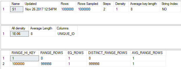
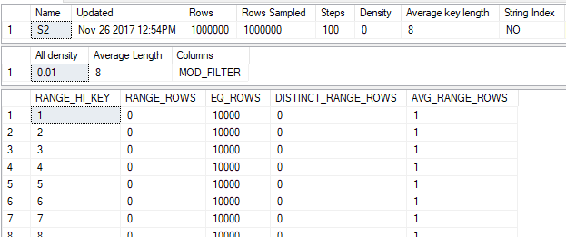
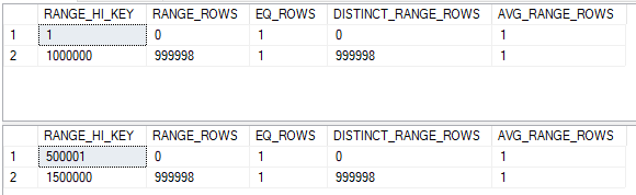
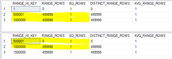
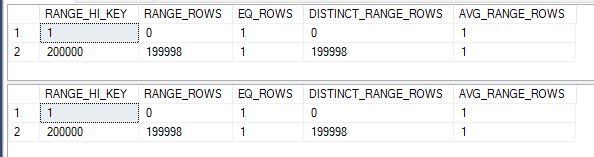
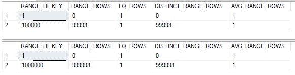
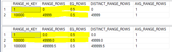
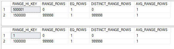
that returned zero rows. However, I wanted the query optimizer to think that a decent number of rows would be returned. This was more difficult to do than expected. I could have just hacked stats to easily accomplish what I wanted, but did not do so out of stubbornness and pride. I eventually found a data set through trial and error with a final cardinality estimate of 16935.2 rows, or 1.7% of the rows in the outer table:

DROP TABLE IF EXISTS dbo.OUTER_HEAP;
CREATE TABLE dbo.OUTER_HEAP (
	ID VARCHAR(10)
);

INSERT INTO dbo.OUTER_HEAP WITH (TABLOCK)
SELECT TOP (1000000) 1500000
	+ ROW_NUMBER() OVER (ORDER BY (SELECT NULL))
FROM master..spt_values t1
CROSS JOIN master..spt_values t2
OPTION (MAXDOP 1);

CREATE STATISTICS S1 ON dbo.OUTER_HEAP (ID)
WITH FULLSCAN;

DROP TABLE IF EXISTS dbo.INNER_CI;
CREATE TABLE dbo.INNER_CI (
	ID VARCHAR(10),
	PRIMARY KEY (ID)
);

INSERT INTO dbo.INNER_CI WITH (TABLOCK)
SELECT TOP (2000000) 500000
	+ ROW_NUMBER() OVER (ORDER BY (SELECT NULL))
FROM master..spt_values t1
CROSS JOIN master..spt_values t2
OPTION (MAXDOP 1);

CREATE STATISTICS S1 ON dbo.INNER_CI (ID)
WITH FULLSCAN;

The actual query of interest is the following one:

SELECT TOP (1) 1
FROM dbo.OUTER_HEAP o
WHERE NOT EXISTS
(
    SELECT 1
    FROM dbo.INNER_CI i
    WHERE i.ID = o.ID
);

Such a query might be used as part of an ETL process as some kind of data validation step. The most interesting case to me is when the query returns no rows, but the query optimizer (for whatever reason) thinks otherwise.

Row Goal Problems

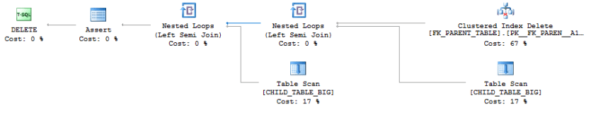
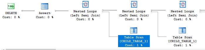
On my machine I get the following plan for the TOP (1) query:

a29_row_goal_nl


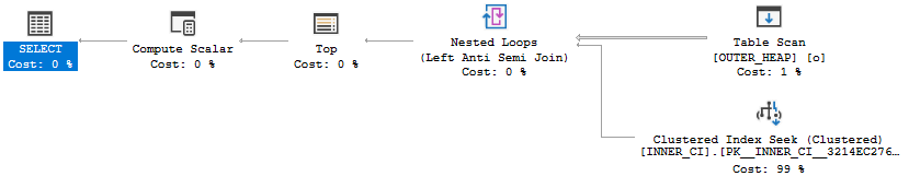
The plan has a total cost of 0.198516 optimizer units. If you know anything about row goals (this may be a good time for the reader to visit Paul White’s series on row goals) you might not be terribly surprised by the outcome. The row goal introduced by the TOP (1) makes the nested loop join very attractive in comparison to other plan choices. The cost of the scan on OUTER_HEAP is discounted from 2.93662 units to 0.0036173 units and the optimizer only expects to do 116 clustered index seeks against INNER_CI before it finds a row that does not match. However, we know our data and we know that all rows match. Therefore, the query will not return any rows and it must scan all rows in OUTER_HEAP if I execute the query. On my machine the query takes about two seconds:

CPU time = 1953 ms, elapsed time = 1963 ms.

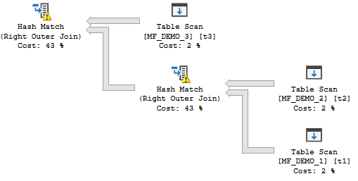
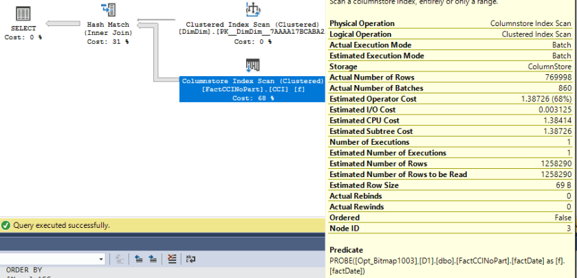
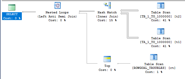
If we’re going to read most of the rows anyway why not try a HASH JOIN hint? At least that plan won’t have a million clustered index seeks:

a29_HJ_PLAN

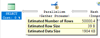
The new plan runs in MAXDOP 4 on my machine (although for not very long due to CPU cooling issues) and has a total cost of 19.9924 optimizer units. Query execution finishes in significantly less time:

CPU time = 1187 ms, elapsed time = 372 ms.

The Riddle

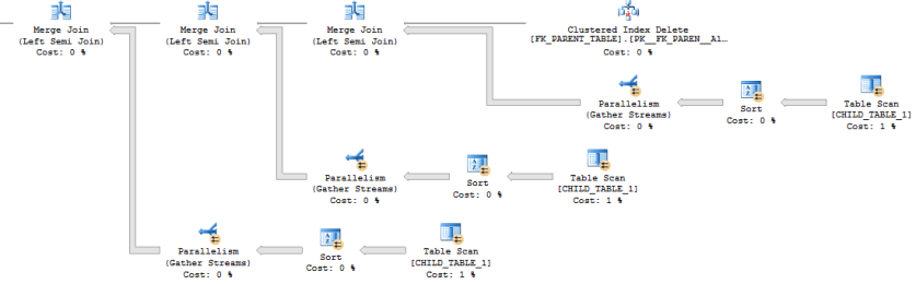
Can we do better than an ugly join hint? Microsoft blessed us with USE HINT functionality in SQL Server 2016 SP1, so let’s go ahead and try that to see if we can improve the performance of the query. To understand the full effect of the hint let’s get estimated plans for OPTION clauses of (USE HINT ('DISABLE_OPTIMIZER_ROWGOAL'), LOOP JOIN) and (USE HINT ('DISABLE_OPTIMIZER_ROWGOAL'), HASH JOIN). In theory, that will make it easy to compare the two queries:

a29_compare_plans

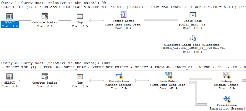
Something looks very wrong here. The loop join plan has a significantly lower cost than the hash join plan! In fact, the loop join plan has a total cost of 0.0167621 optimizer units. Why would disabling row goals for such a plan cause a decrease in total query cost?

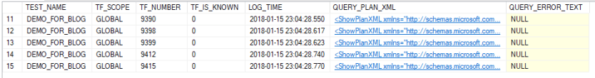
I uploaded the estimated plans here for those who wish to examine them without going through the trouble of creating tables.

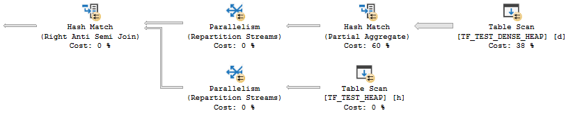
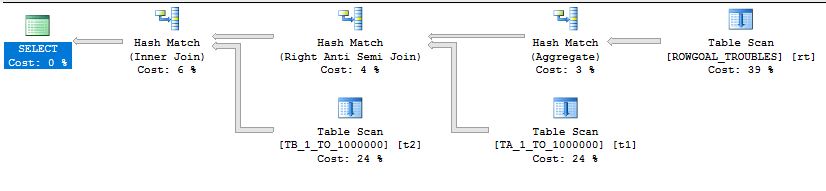
Let’s Try Adding Trace Flags

First let’s try the query with just a USE HINT and no join hint. I get the hash join plan shape that I was after with a total cost of 19.9924 optimizer units. That’s definitely a good thing, but why did the optimizer pick that plan? The plan with a loop join is quite a bargain at 0.0167621 optimizer units. The optimization level is FULL, but that doesn’t mean that every possible plan choice was evaluated. Perhaps the answer is as simple as the optimizer did not consider a nested loop join plan while evaluating possible plan choices.

There are a few different ways to see which optimizer rules were considered during query plan compilation. We can add trace flags 3604 and 8619 at the query level to get information about the rules that were applied during optimization. All of these trace flags are undocumented, don’t use them in production, blah blah blah. For clarity, the query now looks like this:

SELECT TOP (1) 1
FROM dbo.OUTER_HEAP o
WHERE NOT EXISTS
(
    SELECT 1
    FROM dbo.INNER_CI i
    WHERE i.ID = o.ID
) OPTION (USE HINT ('DISABLE_OPTIMIZER_ROWGOAL')
, QUERYTRACEON 3604
, QUERYTRACEON 8619
);

Among other rules, we can see a few associated with nested loops:

Apply Rule: LeftSideJNtoIdxLookup - LOJN/LSJ/LASJ -> IDX LOOKUP
Apply Rule: LASJNtoNL - LASJN -> NL

So the optimizer did consider nested loop joins at some point but it went with the hash join plan instead. That’s interesting.

Let’s Try More Trace Flags

A logical next step is to try to get more operator costing information. Perhaps the cost of the nested loop join plan when considered during optimization is different from the value displayed in the query plan in SSMS. As the optimizer applies different rules and does different transformations the overall cost can change, so I suppose this isn’t a totally unreasonable theory. My first attempt at getting cost information for multiple plan options is by looking at the final memo for the query. This can be done with trace flag 8615.

For clarity, the query now looks like this:

SELECT TOP (1) 1
FROM dbo.OUTER_HEAP o
WHERE NOT EXISTS
(
    SELECT 1
    FROM dbo.INNER_CI i
    WHERE i.ID = o.ID
) OPTION (USE HINT ('DISABLE_OPTIMIZER_ROWGOAL')
, QUERYTRACEON 3604
, QUERYTRACEON 8615
-- , QUERYTRACEON 8619
);

Group 8 is the only one with any costing information for joins:

Group 8: Card=16935.2 (Max=1.1e+006, Min=0)
   11 PhyOp_HashJoinx_jtLeftAntiSemiJoin 6.9 7.10 5.0  Cost(RowGoal 0,ReW 0,ReB 0,Dist 0,Total 0)= 26.5569 (Distance = 1)
   4 PhyOp_HashJoinx_jtLeftAntiSemiJoin 6.4 7.3 5.0  Cost(RowGoal 0,ReW 0,ReB 0,Dist 0,Total 0)= 38.4812 (Distance = 1)
   1 LogOp_RightAntiSemiJoin 7 6 5 (Distance = 1)
   0 LogOp_LeftAntiSemiJoin 6 7 5 (Distance = 0)

This is rather disappointing. There’s only costing information for a few hash join plans. We know that other join types were considered. Perhaps they were discarded from the memo. The final memo just doesn’t have enough information to answer our question.

We Must Not Be Using Enough Trace Flags

There’s a trace flag that adds memo arguments to trace flag 8619: 8620. Perhaps that will give us additional clues. For clarity, the query now looks like this:

SELECT TOP (1) 1
FROM dbo.OUTER_HEAP o
WHERE NOT EXISTS
(
    SELECT 1
    FROM dbo.INNER_CI i
    WHERE i.ID = o.ID
) OPTION (USE HINT ('DISABLE_OPTIMIZER_ROWGOAL')
, QUERYTRACEON 3604
, QUERYTRACEON 8615
, QUERYTRACEON 8619
, QUERYTRACEON 8620
);

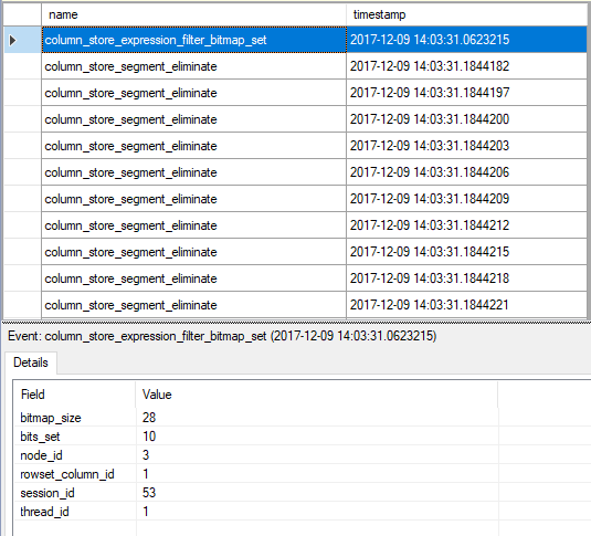
The output is again disappointing. I’ll skip covering it and jump to trace flag 8621. That one adds additional information about the rules and how they interact with memos. With this trace flag we find more information about the plans with merge or loop joins:

Rule Result: group=8 1 LogOp_RightAntiSemiJoin 7 6 5 (Distance = 1)
Rule Result: group=8 2 PhyOp_MergeJoin 1-M x_jtRightAntiSemiJoin 7 6 5 (Distance = 2)
Rule Result: group=8 3 PhyOp_HashJoinx_jtRightAntiSemiJoin 7 6 5 (Distance = 2)
Rule Result: group=8 4 PhyOp_HashJoinx_jtLeftAntiSemiJoin 6 7 5 (Distance = 1)
Rule Result: group=8 5 PhyOp_Applyx_jtLeftAntiSemiJoin 6 16 (Distance = 1)
Rule Result: group=8 6 PhyOp_Applyx_jtLeftAntiSemiJoin 6 16 (Distance = 1)
Rule Result: group=8 7 PhyOp_LoopsJoinx_jtLeftAntiSemiJoin 6 17 5 (Distance = 1)
Rule Result: group=8 8 PhyOp_LoopsJoinx_jtLeftAntiSemiJoin 6 7 5 (Distance = 1)
Rule Result: group=8 9 PhyOp_MergeJoin 1-M x_jtRightAntiSemiJoin 7 6 5 (Distance = 2)
Rule Result: group=8 10 PhyOp_HashJoinx_jtRightAntiSemiJoin 7 6 5 (Distance = 2)
Rule Result: group=8 11 PhyOp_HashJoinx_jtLeftAntiSemiJoin 6 7 5 (Distance = 1)
Rule Result: group=8 12 PhyOp_Applyx_jtLeftAntiSemiJoin 6 16 (Distance = 1)
Rule Result: group=8 13 PhyOp_Applyx_jtLeftAntiSemiJoin 6 16 (Distance = 1)
Rule Result: group=8 14 PhyOp_LoopsJoinx_jtLeftAntiSemiJoin 6 17 5 (Distance = 1)
Rule Result: group=8 15 PhyOp_LoopsJoinx_jtLeftAntiSemiJoin 6 17 5 (Distance = 1)
Rule Result: group=8 16 PhyOp_LoopsJoinx_jtLeftAntiSemiJoin 6 7 5 (Distance = 1)
Rule Result: group=8 17 PhyOp_LoopsJoinx_jtLeftAntiSemiJoin 6 7 5 (Distance = 1)

However, group 8 in the final memo still looks the same as before:

Group 8: Card=16935.2 (Max=1.1e+006, Min=0)
   11 PhyOp_HashJoinx_jtLeftAntiSemiJoin 6.9 7.10 5.0  Cost(RowGoal 0,ReW 0,ReB 0,Dist 0,Total 0)= 26.5569 (Distance = 1)
   4 PhyOp_HashJoinx_jtLeftAntiSemiJoin 6.4 7.3 5.0  Cost(RowGoal 0,ReW 0,ReB 0,Dist 0,Total 0)= 38.4812 (Distance = 1)
   1 LogOp_RightAntiSemiJoin 7 6 5 (Distance = 1)
   0 LogOp_LeftAntiSemiJoin 6 7 5 (Distance = 0)

My interpretation is that costing information for the other join types was discarded from the memo. For example, at one point there was an item 5 in group 8 which contained information relevant to costing for one of the nested loop join plans. All of that information is not present in the final plan because the hash join plan was cheaper.

Pray to the Trace Flag Gods

There is an undisclosed trace flag which does not allow items to be discarded from the memo. Obviously this is a dangerous thing to do. However, with that trace flag group 8 finally reveals all of its secrets:

Group 8: Card=16935.2 (Max=1.1e+006, Min=0)
   17 PhyOp_LoopsJoinx_jtLeftAntiSemiJoin 6 7 5.0 (Distance = 1)
   16 PhyOp_LoopsJoinx_jtLeftAntiSemiJoin 6 7 5.0 (Distance = 1)
   15 PhyOp_LoopsJoinx_jtLeftAntiSemiJoin 6 17 5.0 (Distance = 1)
   14 PhyOp_LoopsJoinx_jtLeftAntiSemiJoin 6 17 5.0 (Distance = 1)
   13 PhyOp_Applyx_jtLeftAntiSemiJoin 6 16 (Distance = 1)
   12 PhyOp_Applyx_jtLeftAntiSemiJoin 6 16 (Distance = 1)
   11 PhyOp_HashJoinx_jtLeftAntiSemiJoin 6.9 7.10 5.0  Cost(RowGoal 0,ReW 0,ReB 0,Dist 0,Total 0)= 26.5569 (Distance = 1)
   10 PhyOp_HashJoinx_jtRightAntiSemiJoin 7.8 6 5 (Distance = 2)
   9 PhyOp_MergeJoin 1-M x_jtRightAntiSemiJoin 7.6 6 5 (Distance = 2)
   8 PhyOp_LoopsJoinx_jtLeftAntiSemiJoin 6 7 5.0 (Distance = 1)
   7 PhyOp_LoopsJoinx_jtLeftAntiSemiJoin 6 17 5.0 (Distance = 1)
   6 PhyOp_Applyx_jtLeftAntiSemiJoin 6 16 (Distance = 1)
   5 PhyOp_Applyx_jtLeftAntiSemiJoin 6 16 (Distance = 1)
   4 PhyOp_HashJoinx_jtLeftAntiSemiJoin 6.4 7.3 5.0  Cost(RowGoal 0,ReW 0,ReB 0,Dist 0,Total 0)= 38.4812 (Distance = 1)
   3 PhyOp_HashJoinx_jtRightAntiSemiJoin 7.3 6.4 5.0  Cost(RowGoal 0,ReW 0,ReB 0,Dist 0,Total 0)= 48.5597 (Distance = 2)
   2 PhyOp_MergeJoin 1-M x_jtRightAntiSemiJoin 7.1 6.2 5.0  Cost(RowGoal 0,ReW 0,ReB 0,Dist 0,Total 0)= 106.564 (Distance = 2)
   1 LogOp_RightAntiSemiJoin 7 6 5 (Distance = 1)
   0 LogOp_LeftAntiSemiJoin 6 7 5 (Distance = 0)

Let’s consider item 5 because it’s one of the more reasonable loop join plan options. Item 5 doesn’t give us direct costing information but it directs us to look to group 16:

Group 16: Card=1 (Max=1, Min=0)
   2 PhyOp_Range 1 ASC  5.0  Cost(RowGoal 0,ReW 0,ReB 999999,Dist 1e+006,Total 1e+006)= 165.607 (Distance = 2)
   1 PhyOp_Range 1 ASC  5.0  Cost(RowGoal 0,ReW 0,ReB 999999,Dist 1e+006,Total 1e+006 s)= 165.607 (Distance = 2)
   0 LogOp_SelectIdx 15 5 (Distance = 1)

We can see a cost of 165.607 for the clustered index seeks on the inner side of the join. If that was the cost used when comparing plans then it explains why the optimizer opted for a hash join over the loop join. We might try looking at a query plan for the following:

DECLARE @TOP INT = 1;

SELECT TOP (@TOP) 1
FROM dbo.OUTER_HEAP o
WHERE NOT EXISTS
(
    SELECT 1
    FROM dbo.INNER_CI i
    WHERE i.ID = o.ID
)
OPTION (OPTIMIZE FOR (@TOP = 987654321)
, LOOP JOIN
, MAXDOP 1);

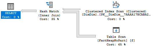
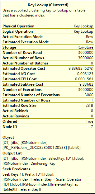
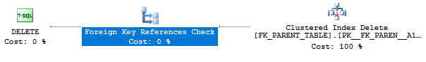
With the above syntax we will get the same query results as before but the effective TOP (1) cannot change the cost of the query. Here are the operator details for the clustered index seek on INNER_CI:

a29_seek_costs

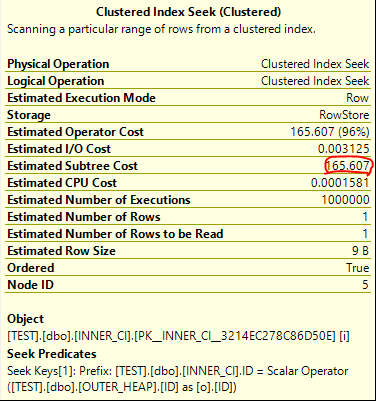
It’s an exact match. The total cost of the query is 172.727 optimizer units, which is significantly more than the price tag of 19.9924 units for the hash join plan.

Improving Displayed Costing

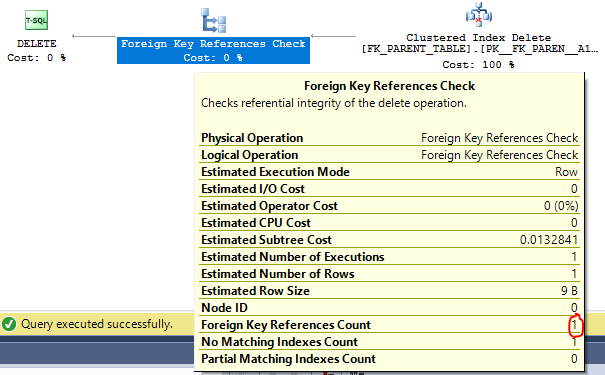
So is there really a problem with the displayed cost of the plan with hints matching (USE HINT ('DISABLE_OPTIMIZER_ROWGOAL'), LOOP JOIN)? After all, the USE HINT seemed to give the correct plan shape without the join hints. Let’s compare the TOP plan side by side with it:

a29_compare_nl_plans

I also uploaded the estimated plans here.

In my view, the costs of the USE HINT plan are nonsensical. The scan and the seeks have matching operator costs of 0.0167621 units. Bizarrely, this also matches the final query cost. 0.0167621 + 0.0167621 = 0.0167621. It’s totally unclear where these numbers come from, and if a TOP (1) can aggressively discount all of the operators in a plan then it seems like the DISABLE_OPTIMIZER_ROWGOAL hint will not have its intended practical impact. Certainly a TOP (1) will not discount the costs of blocking operators, so plans without them (such as loop joins) will be costed cheaper than plans with them (like hash joins).

I would prefer to see matching query costs for both subtrees. Of course, the TOP (1) can influence the costs of other parts of the plan that depend on this subtree, so the estimate needs to obey the TOP expression. I just feel that it shouldn’t affect the cost of the immediate subtree.

If you’re curious where the 0.016762 number comes from, I suspect that it has something to do with the TOP (1) capping the cost of the nested loop join. The following can be found in the final memo:

Group 11: Card=1 (Max=1, Min=0)
   1 PhyOp_Top 8.2 9.0 10.0  Cost(RowGoal 0,ReW 0,ReB 0,Dist 0,Total 0)= 0.016762 (Distance = 1)

Group 8: Card=16935.2 (Max=1.1e+006, Min=0)
   2 PhyOp_Applyx_jtLeftAntiSemiJoin 6.4 15.2  Cost(RowGoal 0,ReW 0,ReB 0,Dist 0,Total 0)= 172.723 (Distance = 1)

In addition, the query cost slightly increases when I change the query to return the first 2 rows. You could argue that query plan costs are just numbers and there’s no reason to care about them as long as you get the right plan, but that’s not quite true. I’m sure this isn’t an exhaustive list, but query plan costs can affect at least the following:

  • If the query cost is too low it won’t be eligible for a parallel plan.
  • The number of seconds that a query will wait for a memory grant before throwing an error.
  • The amount of steps taken by the optimizer during query plan creation.
  • If the query is sent to a small query resource semaphore.
  • If the query is not able to run due to the query governor cost limit.

Final Thoughts

Congrats if you made it to the end. Thanks for reading!

Advertisement

The Return of RESERVED_MEMORY_ALLOCATION_EXT

It is possible to see a scalability bottleneck in the form of high average wait time for the RESERVED_MEMORY_ALLOCATION_EXT wait if a highly concurrent workload is run on a server that consumes memory with batch mode operators. I believe that the severity of the bottleneck depends on unknown factors in the server’s initial memory state and the rate of memory actually used by queries to run batch mode operations. This blog post shares a reproduction of the issue along with a call to action.

The Test Query

Data prep for the test query is very simple. We throw the first ten million sequential integers into two single column BIGINT tables. Additionally, an empty CCI is created to add eligibility for batch mode as desired:

DROP TABLE IF EXISTS DUMMY_CCI;
CREATE TABLE DUMMY_CCI (
	ID INT,
	INDEX CCI CLUSTERED COLUMNSTORE
);

DROP TABLE IF EXISTS HASH_JOIN_SCALE_TEST_1;
CREATE TABLE HASH_JOIN_SCALE_TEST_1 (
	ID BIGINT NOT NULL
);

INSERT INTO HASH_JOIN_SCALE_TEST_1 WITH (TABLOCK)
SELECT TOP (10000000) ROW_NUMBER()
	OVER (ORDER BY (SELECT NULL))
FROM master..spt_values t1
CROSS JOIN master..spt_values t2
CROSS JOIN master..spt_values t3
OPTION (MAXDOP 1);

DROP TABLE IF EXISTS HASH_JOIN_SCALE_TEST_2;
CREATE TABLE HASH_JOIN_SCALE_TEST_2 (
ID BIGINT NOT NULL
);

INSERT INTO HASH_JOIN_SCALE_TEST_2 WITH (TABLOCK)
SELECT TOP (10000000) ROW_NUMBER()
	OVER (ORDER BY (SELECT NULL))
FROM master..spt_values t1
CROSS JOIN master..spt_values t2
CROSS JOIN master..spt_values t3
OPTION (MAXDOP 1);

The SELECT query that we’re going to test with joins them together and returns a count of distinct IDs:

SELECT COUNT(DISTINCT t1.ID)
FROM dbo.HASH_JOIN_SCALE_TEST_1 t1
LEFT OUTER JOIN dbo.HASH_JOIN_SCALE_TEST_2 t2
	ON t1.ID = t2.ID
OPTION (MAXDOP 1);

This is certainly an odd thing to do, but the point of this query is to create a simple test case that uses a bit of memory to create hash tables. Without any indexes on the table we’re very likely to get a hash join. In row mode the query takes about 17 seconds on the test server and uses 1257528 KB of memory.

As far as I can tell this query is a good fit for batch mode. The join is on BIGINT columns and everything except for the rowstore scans can execute in batch mode:

a28_query_plan

Even with the hidden conversions of 20 million rows from row mode to batch mode the query finishes in about 5 seconds. It uses significantly less memory compared to the row mode query: 386112 KB. All of this seems very reasonable.

Testing at Scale

The situation becomes less reasonable once there are many concurrent queries running at once. We go from the batch mode query running in a third of the time of row mode to sometimes running slower. Testing was done with 96 concurrent queries each running queries until 576 total queries were completed. Below is a graph of OS CPU and OS privileged time CPU based on perfmon data:

a28_cpu_graphs

The first third of the graph corresponds to the batch mode workload. CPU never hits 100% and is extremely variable during the run. We also see a high amount of privileged time in the OS. Within SQL Server, we use a total of 222,400,512 KB of query memory. The total wait time for RESERVED_MEMORY_ALLOCATION_EXT can vary, but for this one it was around 11.5 million ms.

The second third of the graph is the part that resets the server memory state. As stated in the introduction, this scalability bottleneck doesn’t always happen and seems to have some kind of dependency on the server’s initial memory state. Here we do a SELECT COUNT(*) on a 1 TB table to add pressure to the rowstore buffer pool.

The final third of the graph corresponds to the row mode workload. CPU jumps to near 100% very quickly and doesn’t waver much during the run. There is very little privileged time in the OS. Within SQL Server, we use a total of 724,336,128 KB of query memory. The wait time for RESERVED_MEMORY_ALLOCATION_EXT is always significantly reduced compared to batch mode. For this run it was around 107k ms.

In conclusion, we see about 1% of memory wait time with the row mode workload compared to the batch mode workload. Usually the row mode workload finishes a little faster than the batch mode one, despite needing over 3X as much total memory and the per-query efficiency advantage of batch mode.

Speculation on the Problem

There may be a hint in the memory management architecture guide:

Starting with SQL Server 2012, SQL Server might allocate more memory than the value specified in the max server memory setting. This behavior may occur when the Total Server Memory (KB) value has already reached the Target Server Memory (KB) setting (as specified by max server memory). If there is insufficient contiguous free memory to meet the demand of multi-page memory requests (more than 8 KB) because of memory fragmentation, SQL Server can perform over-commitment instead of rejecting the memory request.

This behavior is typically observed during the following operations: Large Columnstore index queries.

There are observable differences in how memory is allocated for the same operator when switching from batch mode to row mode. The number of wait events for RESERVED_MEMORY_ALLOCATION_EXT is significantly higher for row mode compared to batch mode. In addition, it remains nearly constant when TF 834 is enabled:

a28_memory_waits

TF 834 appears to fully resolve the scalability issue with batch mode, just like last time. It offers a dramatic improvement in workload completion time:

a28_summary_of_timings

Perhaps some batch mode operators require contiguous free memory for their allocations but the same operation done through row mode does not have that restriction. I can’t go any further than this because I don’t know anything about OS internals or memory management, but it could explain why we see such different behavior between row mode and batch mode.

Use Your Voice

Since SQL Server 2012, Microsoft has listed TF 834 as incompatible with columnstore. There are lots of scary consequences:

  • A non-yielding scheduler error and associated memory dumps in the SQL Server Error log.
  • Columnstore queries trigger severe performance issues.
  • A SQL Server instance triggers access violations when you execute Columnstore queries.
  • You encounter the following error when you run sp_createstats

However, I’ve been told that many of the SQL Server columnstore benchmarks for the TPC-H benchmarks use TF 834. It seems to be a natural fit for columnstore, and there are some workloads (seen in the lab and reproduced in the last two blog posts) where it resolves a key scalability bottleneck which is difficult to address through other means. I have created a feedback item on UserVoice requesting that Microsoft support TF 834 with columnstore.

Final Thoughts

Please provide feedback on the UserVoice item if you are able to do so. Thanks for reading!

Large CCI ETLs Cannot Scale Without TF 834

Large servers may experience a scalability bottleneck related to the RESERVED_MEMORY_ALLOCATION_EXT wait event during loading of columnstore tables. This blog post shares a reproduction of the issue and discusses some test results.

The Test Server

Testing was done on a four socket bare metal server with 24 cores per socket. The server had 1 TB of RAM and storage was provided by a SAN. Within SQL Server, we were able to read data at a peak rate of about 5.5 GB/s. Hyperthreading was disabled, but there aren’t any other nonstandard OS configuration settings that I’m aware of.

SQL Server 2016 SP1 CU7 was installed on Windows Server 2016. Most default settings were retained for this testing, including allowing auto soft-NUMA to break up the 96 schedulers into 12 groups of 8, with 3 per memory node. Max server memory was set to around 800000 MB. The user database had 24 data files, indirect checkpoints weren’t used, and the memory model in use was conventional. No interesting trace flags were enabled, except perhaps for TF 4199. I did grow max server memory to close to the maximum before starting any of the tests.

Testing Code and Method

The workload test loaded the same data from a SQL Server table into 576 CCI target tables. For my testing I used a source table of one million rows. Each session grabs a number from a sequence, loads data into the table corresponding to the sequence number, and continues to do that until there are no more tables to process. This may seem like an odd test to run, but think of it as an abstract representation of a columnstore ETL workload which loads data into partitioned CCIs.

The first step is to define the source table. I created a 50 column table that stored only 0s in all of its rows. There’s nothing particularly special about this choice other that it has a very low disk footprint as a CCI because it compresses so well. On a non-busy system it took around 7.3 seconds to insert one million rows into a CCI. Below is the table definition:

DROP TABLE IF EXISTS CCI_SOURCE;

CREATE TABLE CCI_SOURCE (
ID1 SMALLINT,
ID2 SMALLINT,
ID3 SMALLINT,
ID4 SMALLINT,
ID5 SMALLINT,
ID6 SMALLINT,
ID7 SMALLINT,
ID8 SMALLINT,
ID9 SMALLINT,
ID10 SMALLINT,
ID11 SMALLINT,
ID12 SMALLINT,
ID13 SMALLINT,
ID14 SMALLINT,
ID15 SMALLINT,
ID16 SMALLINT,
ID17 SMALLINT,
ID18 SMALLINT,
ID19 SMALLINT,
ID20 SMALLINT,
ID21 SMALLINT,
ID22 SMALLINT,
ID23 SMALLINT,
ID24 SMALLINT,
ID25 SMALLINT,
ID26 SMALLINT,
ID27 SMALLINT,
ID28 SMALLINT,
ID29 SMALLINT,
ID30 SMALLINT,
ID31 SMALLINT,
ID32 SMALLINT,
ID33 SMALLINT,
ID34 SMALLINT,
ID35 SMALLINT,
ID36 SMALLINT,
ID37 SMALLINT,
ID38 SMALLINT,
ID39 SMALLINT,
ID40 SMALLINT,
ID41 SMALLINT,
ID42 SMALLINT,
ID43 SMALLINT,
ID44 SMALLINT,
ID45 SMALLINT,
ID46 SMALLINT,
ID47 SMALLINT,
ID48 SMALLINT,
ID49 SMALLINT,
ID50 SMALLINT
);

INSERT INTO CCI_SOURCE WITH (TABLOCK)
SELECT
 ID,ID,ID,ID,ID,ID,ID,ID,ID,ID
,ID,ID,ID,ID,ID,ID,ID,ID,ID,ID
FROM (
	SELECT TOP (1000000) 0 ID
	FROM master..spt_values t1
	CROSS JOIN master..spt_values t2
) t;

Next we need a stored procedure that can save off previous test results (as desired) and reset the server for the next test. If a test name is passed in then results are saved to CCI_TEST_RESULTS and CCI_TEST_WAIT_STATS from the previous run. The procedure always recreates all of the target CCI tables, resets the sequence, clears the buffer pool, and does a few other things.

CREATE OR ALTER PROCEDURE [dbo].[CCI_TEST_RESET] (@PreviousTestName NVARCHAR(100) = NULL, @DebugMe INT = 0)
AS
BEGIN
	DECLARE
	@tablename SYSNAME,
	@table_number INT = 1,
	@SQLToExecute NVARCHAR(4000);

	/*
CREATE TABLE CCI_TEST_WAIT_STATS (
	TEST_NAME NVARCHAR(100),
	WAIT_TYPE NVARCHAR(60),
	WAITING_TASKS_COUNT BIGINT,
	WAIT_TIME_MS BIGINT,
	MAX_WAIT_TIME_MS BIGINT,
	SIGNAL_WAIT_TIME_MS BIGINT
);

CREATE TABLE CCI_TEST_RESULTS (
	TEST_NAME NVARCHAR(100),
	TOTAL_SESSION_COUNT SMALLINT,
	TEST_DURATION INT,
	TOTAL_WORK_TIME INT,
	BEST_TABLE_TIME INT,
	WORST_TABLE_TIME INT,
	TOTAL_TABLES_PROCESSED SMALLINT,
	MIN_TABLES_PROCESSED SMALLINT,
	MAX_TABLES_PROCESSED SMALLINT
);
	*/

	SET NOCOUNT ON;

	IF @DebugMe = 0
	BEGIN
		DROP SEQUENCE IF EXISTS CCI_PARALLEL_TEST_SEQ;
		CREATE SEQUENCE CCI_PARALLEL_TEST_SEQ
			AS SMALLINT
			START WITH 1
			INCREMENT BY 1
			CACHE 600;

		IF @PreviousTestName  N''
		BEGIN
			INSERT INTO CCI_TEST_RESULTS WITH (TABLOCK)
			SELECT @PreviousTestName,
			  COUNT(*) TOTAL_SESSION_COUNT
			, DATEDIFF(MILLISECOND, MIN(MIN_START_TIME), MAX(MAX_END_TIME)) TEST_DURATION
			, SUM(TOTAL_SESSION_TIME) TOTAL_WORK_TIME
			, MIN(MIN_TABLE_TIME) BEST_TABLE_TIME
			, MAX(MAX_TABLE_TABLE) WORST_TABLE_TIME
			, SUM(CNT) TOTAL_TABLES_PROCESSED
			, MIN(CNT) MIN_TABLES_PROCESSED
			, MAX(CNT) MAX_TABLES_PROCESSED
			FROM (
				SELECT
				  SESSION_ID
				, COUNT(*) CNT
				, SUM(DATEDIFF(MILLISECOND, START_TIME, END_TIME)) TOTAL_SESSION_TIME
				, MIN(DATEDIFF(MILLISECOND, START_TIME, END_TIME)) MIN_TABLE_TIME
				, MAX(DATEDIFF(MILLISECOND, START_TIME, END_TIME)) MAX_TABLE_TABLE
				, MIN(START_TIME) MIN_START_TIME
				, MAX(END_TIME) MAX_END_TIME
				FROM CCI_TEST_LOGGING_TABLE
				GROUP BY SESSION_ID
			) t;

			INSERT INTO CCI_TEST_WAIT_STATS WITH (TABLOCK)
			SELECT @PreviousTestName, * FROM sys.dm_os_wait_stats
			WHERE wait_type IN (
				'RESERVED_MEMORY_ALLOCATION_EXT'
				, 'SOS_SCHEDULER_YIELD'
				, 'PAGEIOLATCH_EX'
				, 'MEMORY_ALLOCATION_EXT'
				, 'PAGELATCH_UP'
				, 'PAGEIOLATCH_SH'
				, 'WRITELOG'
				, 'LATCH_EX'
				, 'PAGELATCH_EX'
				, 'PAGELATCH_SH'
				, 'CMEMTHREAD'
				, 'LATCH_SH'
			);

		END;

		DROP TABLE IF EXISTS CCI_TEST_LOGGING_TABLE;
		CREATE TABLE CCI_TEST_LOGGING_TABLE (
			SESSION_ID INT,
			TABLE_NUMBER INT,
			START_TIME DATETIME,
			END_TIME DATETIME
		);

	END;

	WHILE @table_number BETWEEN 0 AND 576
	BEGIN
		SET @tablename = N'CCI_PARALLEL_RPT_TARGET_' + CAST(@table_number AS NVARCHAR(3));
		SET @SQLToExecute= N'DROP TABLE IF EXISTS ' + QUOTENAME(@tablename);
		IF @DebugMe = 1
		BEGIN
			PRINT @SQLToExecute;
		END
		ELSE
		BEGIN
			EXEC (@SQLToExecute);
		END;

		SET @SQLToExecute = N'SELECT * INTO ' + QUOTENAME(@tablename) +
		' FROM CCI_SOURCE WHERE 1 = 0';
		IF @DebugMe = 1
		BEGIN
			PRINT @SQLToExecute;
		END
		ELSE
		BEGIN
			EXEC (@SQLToExecute);
		END;

		SET @SQLToExecute = N'CREATE CLUSTERED COLUMNSTORE INDEX CCI ON ' + QUOTENAME(@tablename);
		IF @DebugMe = 1
		BEGIN
			PRINT @SQLToExecute;
		END
		ELSE
		BEGIN
			EXEC (@SQLToExecute);
		END;

		SET @table_number = @table_number + 1;
	END;

	IF @DebugMe = 0
	BEGIN
		DBCC DROPCLEANBUFFERS WITH NO_INFOMSGS;
		DBCC FREEPROCCACHE WITH NO_INFOMSGS;
		DBCC FREESYSTEMCACHE('ALL');

		SELECT COUNT(*) FROM CCI_SOURCE; -- read into cache

		DBCC SQLPERF ("sys.dm_os_wait_stats", CLEAR) WITH NO_INFOMSGS;
		DBCC SQLPERF ("sys.dm_os_spinlock_stats", CLEAR) WITH NO_INFOMSGS;
	END;
END;

Finally we need a stored procedure that can be called to do as many CCI inserts as it can as quickly as possible. I used the following code:

CREATE OR ALTER PROCEDURE [dbo].[CCI_RUN_INSERTS] (@DebugMe INT = 0)
AS
BEGIN
	DECLARE @table_number INT,
	@tablename SYSNAME,
	@SQLToExecute NVARCHAR(4000),
	@start_loop_time DATETIME;

	SET NOCOUNT ON;

	SELECT @table_number = NEXT VALUE FOR CCI_PARALLEL_TEST_SEQ;

	WHILE @table_number BETWEEN 0 AND 576
	BEGIN
		SET @start_loop_time = GETDATE();

		SET @tablename = N'CCI_PARALLEL_RPT_TARGET_' + CAST(@table_number AS NVARCHAR(3));
		SET @SQLToExecute= N'
		INSERT INTO ' + QUOTENAME(@tablename) + N' WITH (TABLOCK)
		SELECT * FROM CCI_SOURCE WITH (TABLOCK)
		OPTION (MAXDOP 1)';

		IF @DebugMe = 1
		BEGIN
			PRINT @SQLToExecute;
		END
		ELSE
		BEGIN
			EXEC (@SQLToExecute);

			INSERT INTO CCI_TEST_LOGGING_TABLE VALUES (@@SPID, @table_number, @start_loop_time, GETDATE());
		END;

		SELECT @table_number = NEXT VALUE FOR CCI_PARALLEL_TEST_SEQ;
	END;
END;

To vary the number of concurrent queries I used sqlcmd. Each set of 12 sessions had the following format:

START /B sqlcmd -d your_db_name -S your_server_name -Q "EXEC dbo.[CCI_RUN_INSERTS]" > nul
ping 192.2.0.1 -n 1 -w 1 > nul

My workflow was to perform this test was to add the desired number of calls to the stored procedure in the .bat file, run the test, and to check the results to make sure that the test was a good one. If it was I saved off results using the reset procedure. If not I ran the reset procedure and tried again.

The ping command is there to add a small delay between sets of queries. I found that adding such a delay led to less doubling up on schedulers. I picked 12 because that’s the number of soft-NUMA nodes. Sometimes tests would get quite a bit of SOS_SCHEDULER_YIELD waits which would mean that they couldn’t be accurately compared to other tests. My fix was to just run the test again. It required a bit of patience but I never had to run a test more than once. SOS waits weren’t eliminated but I’d say they fell to acceptable levels:

a27_SOS_CPU_wait_table

The right way to avoid SOS waits for testing like this (which might require every user session to go on its own scheduler) would be to set up 96 manual soft-NUMA nodes. But who has time for that?

Test Results

12 tests with different numbers of active queries were run. I picked numbers that somewhat evenly divided into 576 to try to keep work balanced between threads. The blue line in the chart below measures how long each test took from start to finish and the orange line represents how fast the test could have completed if there was no contention on the server whatsoever:

a27_No_T834_compare_chart

Naturally we can’t expect the two lines to match perfectly, but improvements in runtime stop after going past 32 threads. In fact, the workload takes longer with 96 threads compared to 32 threads.

The dominant wait event for the higher thread count runs is RESERVED_MEMORY_ALLOCATION_EXT. Below is a chart of all of the wait events worth mentioning for the 96 thread run:

a27_no_T834_wait_table

The total number of wait events for RESERVED_MEMORY_ALLOCATION_EXT is very consistent between runs. However, the average wait time significantly increases as the number of concurrent queries increases:

a27_memory_waits_chart

In fact, it could be said that that nearly all worker time past 32 threads is spent waiting on memory. The final column in the chart below is the total time spent in SQL Server minus wait time for RESERVED_MEMORY_ALLOCATION_EXT. The values in that column are remarkably consistent.

a27_No_TF_834_summary

In my experience, when we get into a situation with high memory waits caused by too much concurrent CCI activity all queries on the server that use a memory grant can be affected. For example, I’ve seen sp_whoisactive run for longer than 90 seconds.

It needs to be stated that not all CCIs will suffer from this scalability problem. I was able to achieve good scalability with some artificial tables, but all of the real target tables that I tested have excessive memory waits at high concurrency. Perhaps tables which require more CPU to compress naturally spread out their memory requests and the underlying OS is better able to keep up.

Test Results With Trace Flag 834

Microsoft strongly recommends against using trace flag 834 with columnstore tables. There’s even an article dedicated to that warning. I was desperate so I tried it anyway. The difference was night and day:

a27_T834_compare_chart

Enabling trace flag 834 does at least three things: SQL Server grows to max server memory on startup, AWE memory is used for memory access, and large pages are used for the buffer pool. I didn’t see gains when using LPIM (which uses AWE memory) or by growing memory to max before running tests with a conventional memory model, so I suspect that the large pages are making a key difference. Wait time for RESERVED_MEMORY_ALLOCATION_EXT is under a second for all tests.

Scalability is diminished a bit for the 96 thread run. There are some wait events that creep up:

TF_834_96_thread_wait_stats

All of the wait events can be troubleshooted in conventional ways except possibly for CMEMTHREAD. There’s no longer a large amount of time spent outside of SQL Server in the OS.

Other Workarounds

Without trace flag 834 this can be a difficult problem to work around. The two main strategies are to spread out CCI insert activity as much as possible during the ETL and to reduce memory usage of queries which run at the same time as the CCI inserts. For example, consider a query that inserts into a CCI that also performs a large hash join. If that hash join can be moved to somewhere else in the process then you might come out ahead in reducing contention on memory.

Other than that, there’s some evidence that virtualized servers are not a good fit for this type of workload. Large virtual guests experience the memory waits at an increased rate, but it isn’t yet clear if the problem can be avoided through some change in VM configuration.

Final Thoughts

It’s hard not to conclude that TF 834 is necessary to get scalability for columnstore ETLs on very large servers. Hopefully Microsoft will make TF 834 compatible with columnstore one day in the future. Thanks for reading!

Batch Mode Memory Fractions

My least favorite tempdb spills are the ones that happen with a large percentage of the memory grant remaining unused. For example, recently I saw tempdb spills with a memory grant of 35 GB but SQL Server reported that only 10 GB of memory was used. Usually this problem can be traced back to suboptimal memory fractions somewhere in a query plan. I suspect that it can also happen with certain types of queries that load data into columnstore tables but haven’t verified that. In the test environment the issue was caused by memory fractions, but these memory fractions were attached to batch mode operators. The rules for batch mode memory fractions certainly appear to be different than those for rowstore memory fractions. I believe that I was able to work out a few of the details for a few simple cases. In some scenarios, plans with multiple batch mode hash joins can ask for significantly more memory than needed. Reducing the memory grant via Resource Governor or a query hint to something more reasonable can lead to unnecessary (and often frustrating) tempdb spills.

What is a Memory Fraction?

There’s very little information out there about memory fractions. I would define them as information in the query plan that can give you clues about each operator’s share of the total query memory grant. This is naturally more complicated for query plans that insert into tables with columnstore indexes but that won’t be covered here. Most references will tell you not to worry about memory fractions or that they aren’t useful most of the time. Out of thousands of queries that I’ve tuned I can only think of a few for which memory fractions were relevant. Sometimes queries spill to tempdb even though SQL Server reports that a lot of query memory was unused. In these situations I generally hope for a poor cardinality estimate which leads to a memory fraction which is too low for the spilling operator. If fixing the cardinality estimate doesn’t prevent the spill then things can get a lot more complicated, assuming that you don’t just give up.

Types of Query Plans

The demos for this blog post all use tables with identical structures and data. The tables are heaps so the plans will only feature hash joins. The most important plan characteristic is how many of the hash tables need to be kept in memory concurrently while the query processor executes the query. This is where memory fractions come in. The query optimizer tries to reuse parts of memory grants as it can. For example, if the hash build for the first join isn’t needed when the third join executes then it’s possible to use the memory grant from the first hash table for the third hash table. Some of the examples below will make this more clear.

The first type of plan has hash joins which can all run concurrently. Memory for the hash tables cannot be reused between operators.

a26_concurrent_joins

For that query, the MF_DEMO_1 table is the probe side for all of the joins. SQL Server builds all of the hash joins and then rows flow from the probe side through the plan (as long as there aren’t tempdb spills). I will refer to this type of plan as a “concurrent join plan” which is a term that I just made up.

The second type of plan has hash joins which cannot all run concurrently. Pairs of hash tables are active at the same time, but memory grants can be reused between operators.

s26_nonconcurrent_joins

For that query, the MF_DEMO_1 table is the build side for all of the joins. Each hash table blocks the next one from starting. This means that at most two hash tables need to be kept in memory at the same time. Query memory cannot be reused for joins 1 and 2 but join 3 can reuse memory from join 1 and join 4 can reuse memory from join 2. I will refer to this type of plan as a “nonconcurrent join plan” which is another term that I just made up.

If the above wasn’t clear I recommend running through the demos with live query statistics enabled. It can be very useful to understand how rows flow through a plan. As far as I know, all queries of this type can be implemented with the nonconcurrent pattern but not all queries can be implemented with the concurrent pattern .

Create the Tables

The table definitions for our demos are pretty boring. I’m using a VARCHAR(100) as the join column to blow up memory grants and requirements a bit. All of the tables are heaps and have about 6.5 million rows in them. TARGET_TABLE is used as a dumping ground for the inserts and #ADD_BATCH_MODE is used to switch the hash joins to batch mode as desired. All testing was done on SQL Server 2016 SP1 CU7.

DROP TABLE IF EXISTS MF_DEMO_1;
CREATE TABLE MF_DEMO_1 (
       ID VARCHAR(100)
);

INSERT INTO MF_DEMO_1 WITH (TABLOCK)
SELECT 999999999999999 + ROW_NUMBER()
	OVER (ORDER BY (SELECT NULL))
FROM master..spt_values t1
CROSS JOIN master..spt_values t2;

CREATE STATISTICS S1 ON MF_DEMO_1 (ID) WITH FULLSCAN;

DROP TABLE IF EXISTS MF_DEMO_2;
CREATE TABLE MF_DEMO_2 (
       ID VARCHAR(100)
);

INSERT INTO MF_DEMO_2 WITH (TABLOCK)
SELECT 999999999999999 + ROW_NUMBER()
	OVER (ORDER BY (SELECT NULL))
FROM master..spt_values t1
CROSS JOIN master..spt_values t2;

CREATE STATISTICS S2 ON MF_DEMO_2 (ID) WITH FULLSCAN;

DROP TABLE IF EXISTS MF_DEMO_3;
CREATE TABLE MF_DEMO_3 (
       ID VARCHAR(100)
); 

INSERT INTO MF_DEMO_3 WITH (TABLOCK)
SELECT 999999999999999 + ROW_NUMBER()
	OVER (ORDER BY (SELECT NULL))
FROM master..spt_values t1
CROSS JOIN master..spt_values t2;

CREATE STATISTICS S3 ON MF_DEMO_3 (ID) WITH FULLSCAN;

DROP TABLE IF EXISTS MF_DEMO_4;
CREATE TABLE MF_DEMO_4 (
       ID VARCHAR(100)
); 

INSERT INTO MF_DEMO_4 WITH (TABLOCK)
SELECT 999999999999999 + ROW_NUMBER()
	OVER (ORDER BY (SELECT NULL))
FROM master..spt_values t1
CROSS JOIN master..spt_values t2;

CREATE STATISTICS S4 ON MF_DEMO_4 (ID) WITH FULLSCAN;

DROP TABLE IF EXISTS MF_DEMO_5;
CREATE TABLE MF_DEMO_5 (
	ID VARCHAR(100)
); 

INSERT INTO MF_DEMO_5 WITH (TABLOCK)
SELECT 999999999999999 + ROW_NUMBER()
	OVER (ORDER BY (SELECT NULL))
FROM master..spt_values t1
CROSS JOIN master..spt_values t2;

CREATE STATISTICS S5 ON MF_DEMO_5 (ID) WITH FULLSCAN;

CREATE TABLE #ADD_BATCH_MODE (I INT, INDEX CCI CLUSTERED COLUMNSTORE);

DROP TABLE IF EXISTS TARGET_TABLE;

CREATE TABLE TARGET_TABLE (ID VARCHAR(100));

Row Mode Memory Fractions For Concurrent Join Plans

The following query results in a concurrent join plan with row mode hash joins:

INSERT INTO TARGET_TABLE WITH (TABLOCK)
SELECT t1.ID
FROM MF_DEMO_3 t3
RIGHT OUTER JOIN MF_DEMO_2 t2
RIGHT OUTER JOIN MF_DEMO_1 t1
ON t1.ID = t2.ID
ON t1.ID = t3.ID
OPTION (FORCE ORDER, MAXDOP 1);

The desired memory grant is 2860640 KB. The memory fractions for both join operators have an input of 0.5 and an output of 0.5. This is exactly as expected. The hash tables can both start at the same time and cannot reuse memory, so each operator gets 50% of the query memory grant for the plan. Adding a third join to the plan increases the query memory grant to 4290960 KB.

INSERT INTO TARGET_TABLE WITH (TABLOCK)
SELECT t1.ID
FROM MF_DEMO_4 t4
RIGHT OUTER JOIN MF_DEMO_3 t3
RIGHT OUTER JOIN MF_DEMO_2 t2
RIGHT OUTER JOIN MF_DEMO_1 t1
ON t1.ID = t2.ID
ON t1.ID = t3.ID
ON t1.ID = t4.ID
OPTION (FORCE ORDER, MAXDOP 1);

Again, this seems very reasonable. SQL Server now tries to builds three hash tables in memory at the same time. The memory fractions for each operator have fallen to 0.3333333. Each operator gets a third of the query memory grant.

Row Mode Memory Fractions For Nonconcurrent Join Plans

The following query results in a nonconcurrent join plan with row mode hash joins:

INSERT INTO TARGET_TABLE WITH (TABLOCK)
SELECT t1.ID
FROM MF_DEMO_1 t1
INNER JOIN MF_DEMO_2 t2 ON t1.ID = t2.ID
INNER JOIN MF_DEMO_3 t3 ON t2.ID = t3.ID
INNER JOIN MF_DEMO_4 t4 ON t3.ID = t4.ID
OPTION (MAXDOP 1, FORCE ORDER);

The query plan was uploaded here. I recommend downloading the all of the plans referenced in this blost post if you’re interested in them so you can see all of the details.

Here are the memory fractions for the rightmost join (node 3):

Memory Fractions Input: 1, Memory Fractions Output: 0.476174

here are the memory fractions for the middle join (node 2):

Memory Fractions Input: 0.523826, Memory Fractions Output: 0.5

and here are the memory fractions for the leftmost join (node 1):

Memory Fractions Input: 0.5, Memory Fractions Output: 1

What do all of those numbers mean? The rightmost join builds its hash table first and starts with all query memory available to it. However, the output fraction is 0.476174. That means that the hash table can only use up to 47.6% of the query memory granted to the plan. The middle join is able to use up to 50% (the minimum of the input and output fractions for the node) of the memory granted to the plan. Note that 0.476174 + 0.523826 = 1.0. The last join to start executing is also able to use up to 50% of the granted memory. That join is the last operator that uses memory in the plan so the output fraction is 1.0. Memory grant reuse allows the plan to use up to 147.6% of the memory grant over the lifetime of the query execution. Without memory grant reuse each operator wouldn’t be able to use as much memory.

Removing one of the joins results in the desired query memory grant dropping from 3146704 KB to 3003672 KB. This is a significantly less drop than the other query. The smaller decrease is expected because the third join that we added can reuse the memory grant from the first. As more joins are added to a nonconcurrent plan the desired memory grant grows at a much slower rate than the memory grant for the concurrent join plan.

Batch Mode Memory Fractions For Concurrent Join Plans

The query plan for the next query is somewhat dependent on hardware. On my machine I had to let it run in parallel to get batch mode hash joins:

INSERT INTO TARGET_TABLE WITH (TABLOCK)
SELECT t1.ID
FROM MF_DEMO_5 t5
RIGHT OUTER JOIN MF_DEMO_4 t4
RIGHT OUTER JOIN MF_DEMO_3 t3
RIGHT OUTER JOIN MF_DEMO_2 t2
RIGHT OUTER JOIN MF_DEMO_1 t1
LEFT OUTER JOIN #ADD_BATCH_MODE ON 1 = 0
ON t1.ID = t2.ID
ON t1.ID = t3.ID
ON t1.ID = t4.ID
ON t1.ID = t5.ID
OPTION (FORCE ORDER, MAXDOP 4);

The estimated plan is here. It’s easy to tell if the query is using batch mode joins because the joins are run in parallel but there are no repartition stream operators.

a26_concurrent_joins_batch

SQL Server is not able to reuse memory grants for this query. SQL Server tries to build all of the hash tables in memory before probe side is processed. However, the memory fractions are different from before: 0.25, 0.5, 0.75, and 1.0. These memory fractions do not make sense if interpreted in the same way as before. How can the final hash join in the plan have an input memory fraction of 1.0?

It’s unclear what the memory fractions are supposed to mean here, but there is one observable difference compared to the row mode plan. In the row mode equivalent plan SQL Server divides the memory evenly between operators. For our very simple test plan this means that all of the hash joins will spill to tempdb or none of them will spill. Reducing a MAX_GRANT_PERCENT hint from the right value by 1% results in two spills:

a26_row_mode_spill

Both operators spilled because memory was divided evenly and there wasn’t enough memory to hold both hash tables in memory. However, with batch mode hash joins we can get plans like the following:

a26_batch_spill

How is it possible that one join spills but the other doesn’t? It is only possible if memory isn’t divided evenly. It appears that memory is used as needed in some situations. Unfortunately, the actual plan for batch mode operators doesn’t give us a lot of spill information like it does for row mode. There’s a debug channel extended event query_execution_batch_hash_join_spilled that can give us some clues. 657920 KB of memory was granted for a two batch mode hash join query. For the operator that spilled, only 44852457 bytes were written to memory on the build side. That’s about 43800 KB, which is significantly less than half of available query memory.

a26_concurrent_spill_XE

We can’t conclude that exactly 44852457 bytes of memory were granted to the operator. However, it should be somewhat close. In conclusion, for these types of queries it isn’t clear what the memory grant fractions are supposed to mean. SQL Server is able to exceed them in some cases. It’s possible to see 0 bytes of memory used for the build side in the extended event. I believe that this is the bad type of memory reuse as opposed to the good kind.

Batch Mode Memory Fractions For Nonconcurrent Join Plans

The following query results in a nonconcurrent batch mode hash join plan on my machine:

INSERT INTO TARGET_TABLE WITH (TABLOCK)
SELECT t1.ID
FROM MF_DEMO_1 t1
LEFT OUTER JOIN #ADD_BATCH_MODE On 1 = 0
WHERE EXISTS (
	SELECT 1
	FROM MF_DEMO_2 t2 WHERE t1.ID = t2.ID
) AND EXISTS (
	SELECT 1
	FROM MF_DEMO_3 t3 WHERE t1.ID = t3.ID
) AND EXISTS (
	SELECT 1
	FROM MF_DEMO_4 t4 WHERE t1.ID = t4.ID
) AND EXISTS (
	SELECT 1
	FROM MF_DEMO_5 t5 WHERE t1.ID = t5.ID
) OPTION (MAXDOP 4, FORCE ORDER);

As far as I know there’s nothing special about the semijoins. I used them to keep the estimated row size as consistent as possible. The behavior detailed below can be observed with normal joins as well.

Here is the estimated query plan. The same memory fraction pattern of 0.25, 0.50, 0.75, and 1.00 can be found in this query. Based on the query’s structure, memory grant reuse should be allowed between operators. Alarmingly, this query has the same desired memory grant as one with four concurrent joins. The desired memory grant changes significantly as tables are added or removed. This is a big change in behavior compared to row mode batch joins.

As far as I can tell, memory grant reuse can happen in plans like this with batch mode hash joins. Removing or adding joins results in very small adjustments in maximum memory used during query execution. Still, it seems as if the query optimizer is assuming that memory cannot be reused. With this query pattern, the first operator to run does not have access more memory implied by the memory fraction. In fact, it has access to less memory implied by the memory fraction.

Running the query without any memory grant hints results in no tempdb spills and a maximum memory use of 647168 KB. Restricting the memory grant to 2 GB results in a tempdb spill for the rightmost operator. This is unexpected. 500000 KB of memory should be more than enough memory to avoid a spill. As before, the only way I could find to investigate this further was to use the query_execution_batch_hash_join_spilled extended event and to force tempdb spills using the MAX_GRANT_PERCENT query hint.

A good amount of testing suggested that the available memory per operator is the input memory fraction for that operator divided by the sum of all output memory fractions. The rightmost operator only gets 0.25 / (0.25 + 0.5 + 0.75 + 1.0) = 10% of the memory granted to the query, the next operator gets 20%, the next operator gets 30%, and the final operator gets 40%. The situation gets worse as more joins are added to the query. Keep in mind that we aren’t doing anything tricky with cardinality estimates or data types which would result in skewed estimates. The query optimizer seems to recognize that each join will require the same amount of memory for each hash join, but it doesn’t make the same minimum amount available for each operator. That’s what is so puzzling.

The preceding paragraph seems to contradict the idea that memory grant reuse is possible for these plan shapes. Perhaps for these simple plans memory grant reuse is possible but it cannot go above 100% like we saw in the row mode plan. This could still be helpful in that the query could steal less memory from the buffer pool, but it’s certainly not as helpful in avoiding spills as the behavior we get with the row mode plan. Under the assumption the total memory grants seem a bit more reasonable, although it’s hard not to object as to how SQL Server is distributing the memory to each operator.

We can avoid the spill by giving SQL Server the memory that it required, but this is undesirable if multiple concurrent queries are running. I’ve often observed higher than expected memory grants for queries with batch mode hash joins. An assumption that query memory reuse will not be available for batch mode hash joins can explain part of what I’ve observed. If memory grants are left unchecked, applications may see decreased possible concurrency due to RESOURCE_SEMAPHORE waits. Lowering memory grants through any available method can result in unnecessary (based on total memory granted) tempdb spills. It’s easy to get stuck between a rock and a hard place.

Batch Mode Workarounds

There is some hope for nonconcurrent batch mode hash join plans. SQL Server 2017 introduces adaptive memory feedback for these operators. I imagine that functionality is a poor fit for ETL queries which may process dramatically different amounts of data each day, so I can’t view it as a complete solution. It certainly doesn’t help us on SQL Server 2016. Are there workarounds to prevent spills without requiring excessive memory grants? Yes, but they are very ugly and I can only imagine using them when truly needed during something like an ETL process.

Consider the following query:

INSERT INTO TARGET_TABLE WITH (TABLOCK)
SELECT t1.ID
FROM MF_DEMO_1 t1
LEFT OUTER JOIN MF_DEMO_2 t2 ON t2.ID = t1.ID
LEFT OUTER JOIN MF_DEMO_3 t3 ON t3.ID = t2.ID
LEFT OUTER JOIN MF_DEMO_4 t4 ON t4.ID = t3.ID
LEFT OUTER JOIN MF_DEMO_4 t5 ON t5.ID = t4.ID
LEFT OUTER JOIN #ADD_BATCH_MODE ON 1 = 0
OPTION (FORCE ORDER, MAXDOP 4, MAX_GRANT_PERCENT = 60);

On my machine, the memory hint results in a memory grant of 2193072 KB. The rightmost join spills even when only a maximum of 1232896 KB of memory is used during query execution:

a26_workaround_spill

One way to avoid the spill is to shift the memory fractions in our favor. Ideally SQL Server would think that the rightmost join would need much more memory for its hash table than the other joins. If we can add an always NULL column with a large data type that is only needed for the first hash table, that might do the trick. The query syntax below isn’t guaranteed to get the plan that we want but it seems to work in this case:

ALTER TABLE MF_DEMO_1 ADD DUMMY_COLUMN_V4000 VARCHAR(4000) NULL;
ALTER TABLE MF_DEMO_2 ADD DUMMY_COLUMN_V10 VARCHAR(10) NULL;

INSERT INTO TARGET_TABLE WITH (TABLOCK)
SELECT t1.ID
FROM MF_DEMO_1 t1
LEFT OUTER JOIN MF_DEMO_2 t2 ON t2.ID = t1.ID
LEFT OUTER JOIN MF_DEMO_3 t3 ON t3.ID = t2.ID
LEFT OUTER JOIN MF_DEMO_4 t4 ON t4.ID = t3.ID
LEFT OUTER JOIN MF_DEMO_4 t5 ON t5.ID = t4.ID
LEFT OUTER JOIN #ADD_BATCH_MODE ON 1 = 0
WHERE (t1.DUMMY_COLUMN_V4000 IS NULL OR t2.DUMMY_COLUMN_V10 IS NULL)
OPTION (FORCE ORDER, MAXDOP 4, MAX_GRANT_PERCENT = 32);

An actual plan was uploaded here. The query no longer spills even though the memory grant was cut to 1225960 KB. The memory fractions are now 0.82053, 0.878593, 0.936655, and 1. The change was caused by the increase in estimated row size for the rightmost join: 2029 bytes. That row size is reduced to 45 bytes after the filter is applied, which won’t filter out any rows because both columns are always NULL. The FORCE ORDER hint is essential to get this plan shape. It’s very unnatural otherwise.

If the same rules are followed as before, the rightmost join should get 22.5% of the available query memory grant now. This is enough to avoid the spill to tempdb.

Final Thoughts

I understand that the formulas for memory fractions need to account for an arbitrary combination of row mode and batch mode operators in a query plan. However, it is disappointing that the available information for memory fractions for batch mode operators is so confusing, some queries with batch mode hash joins ask for way more memory than they need, and some queries needlessly spill to tempdb without using close to their full memory grant. Batch mode adaptive memory grant feedback can offer some relief in SQL Server 2017, but why not expect good plans the first time as long as we’re giving the query optimizer good information? Thanks for reading!

A Method to Find Trace Flags

Trace flags are often-hidden configuration switches within SQL Server that can be used to change advanced configuration options, enable or disable fixes, or provide additional diagnostic information. Microsoft recently (on the time scale of the product) published a list of supported trace flags.  The community has found other, undocumented trace flags through various means. The best repository that I’m aware of is maintained by Konstantin Ktaranov here and published here. This blog post contains a stored procedure that can find trace flags. The code contained in this blog post is extremely dangerous and should never be run in production. Be prepared to say goodbye to any server that you run it on.

Hunting Technique

Microsoft gives us a few clues about the range of valid trace flags. All of the documented trace flags (other than the one to make trace flags globally scoped, -1) are positive integers less than 11025. Looking through the list, we can see that similar trace flags are often grouped together. However, the most important hint is that DBCC TRACEON and DBCC TRACEOFF threw an error for any trace flag that’s above some hardcoded maximum. In SQL Server 2017 CU2 the largest allowed value is 11498. What if we had a stored procedure which could take a query to run, turn on one trace flag at a time from 1 to 11498, save off the XML from the estimated plan, turn off the trace flag, go to the next one, and compare all of the generated XML? That would give us a way to check for changes to the XML for everything in the known range of possible trace flags.

The technique described above will not work for trace flags that can only be activated at server startup. You’ll need something like Brent’s method here for that. It also won’t work well for trace flags which need other trace flags to be enabled at the same time. Some trace flags have an effect which cannot be observed through an estimated plan, such as some server settings and aggregate pushdown for CCIs. Still, with the right test query and a little patience you can get some interesting results.

Prepare for the Hunt

The stored procedure requires a few tables to exist and be populated. There is a set of three tables that exclude trace flags in different ways:

CREATE TABLE dbo.STACK_DUMP_TFS (TF INT, PRIMARY KEY (TF));

CREATE TABLE dbo.TFS_TO_EXCLUDE (TF INT, PRIMARY KEY (TF));

CREATE TABLE dbo.KNOWN_TFS (TF INT, PRIMARY KEY (TF));

The first table, STACK_DUMP_TFS, contains trace flags that cause stack dumps which you never want to enable. I found two such trace flags during my testing, but there could be others depending on server configuration and the query that you’re testing. The TFS_TO_EXCLUDE table contains trace flags that you don’t want to enable for one reason or another. Maybe you want to enable a trace flag throughout the lifetime of a test or you’ve found a previously unknown trace flag and you don’t want to continue to show up your test results. The KNOWN_TFS table contains all trace flags found in Konstantin’s trace flag guide. Of course, you can populate the tables with whatever you want, but I put code to populate the tables with the dataset that I use on pastebin.

Finally, the stored procedure logs what it finds to the following table:

CREATE TABLE dbo.LOG_TF_XML_COMPARE (
	TEST_NAME VARCHAR(100) NOT NULL,
	TF_SCOPE VARCHAR(10) NOT NULL,
	TF_NUMBER INTEGER NOT NULL,
	TF_IS_KNOWN INT,
	LOG_TIME DATETIME,
	QUERY_PLAN_XML XML,
	QUERY_ERROR_TEXT NVARCHAR(4000),
	PRIMARY KEY (TEST_NAME, TF_SCOPE, TF_NUMBER)
);

The structure of the table will make more sense after I go through an example later on in this post.

Set Your Bait

The stored procedure has a few parameters to define the search:

@test_name VARCHAR(100),
@query_text NVARCHAR(3900),
@tf_scope VARCHAR(10) = 'GLOBAL',
@first_TF_to_search INT = 1,
@last_TF_to_search INT = 11498,
@skip_known_TFs INT = 1

The @test_name parameter controls what is logged to the TEST_NAME column of LOG_TF_XML_COMPARE. The stored procedure deletes all existing data from the table with a matching @test_name and @tf_scope.

The @query_text parameter contains the query for which an estimated plan to be generated. Currently, the procedure only supports single statement queries, so you can’t define a variable or create a table in the query text and do something else after.

The @tf_scope parameter controls if the trace flags are enabled at the session, global, or query level with QUERYTRACEON. Allowed inputs are 'GLOBAL', 'SESSION', and 'QUERY'. The query level can only be used if @query_text contains a '{{QUERYTRACEON}}' or '{{QUERYHINT}}' placeholder. '{{QUERYTRACEON}}' should be used as a substitute for QUERYTRACEON in the query and '{{QUERYHINT}}' should be used to create the OPTION part of a query, so you’d only use '{{QUERYTRACEON}}' if you need to specify other hints at the query level.

@first_TF_to_search is the first trace flag to search with a default value of 1. Trace flags are always searched in ascending order.

@last_TF_to_search is the last trace flag to search with a default value of 11498. I haven’t done any testing on lower versions of SQL Server, so it’s possible that you’ll see errors when trying trace flags with a higher value on some product versions.

If @skip_known_TFs is set to 0 then trace flags in the KNOWN_TFS table will be skipped during the stored procedure run. Trace flags in the STACK_DUMP_TFS and TFS_TO_EXCLUDE tables are always skipped.

Begin the Hunt

The procedure enables a trace flag, generates a cached plan, does some cleanup on the plan, and saves it into the logging table if it’s different from the plan without any trace flags. The full code of the procedure is below:

-- THIS CODE DOES BAD THINGS!!!!
CREATE OR ALTER PROCEDURE [dbo].[FIND_TRACE_FLAGS] (
@test_name VARCHAR(100),
@query_text NVARCHAR(3900),
@tf_scope VARCHAR(10) = 'GLOBAL',
@first_TF_to_search INT = 1,
@last_TF_to_search INT = 11498,
@skip_known_TFs INT = 1
)
AS
BEGIN
DECLARE
	@plan_handle VARBINARY(64),
	@plan_xml XML,
	@query_error nvarchar(4000),
	@TF INT,
	@trace_sql VARCHAR(1000),
	@standard_plan_xml_as_string NVARCHAR(MAX),
	@TF_is_known INT,
	@query_text_to_run_w_placeholders NVARCHAR(4000),
	@query_text_to_run NVARCHAR(4000)

;
SET NOCOUNT ON;

IF @tf_scope NOT IN ('GLOBAL', 'SESSION', 'QUERY')
BEGIN
	THROW 50001, 'Fix @tf_scope', 1;
	RETURN;
END;

IF @tf_scope = 'QUERY' AND @query_text NOT LIKE '%{{QUERYTRACEON}}%' AND @query_text NOT LIKE '%{{QUERYHINT}}%'
BEGIN
	THROW 50001, '@query_text needs {{QUERYTRACEON}} or {{QUERYHINT}} placeholder', 1;
	RETURN;
END;

IF @first_TF_to_search NOT BETWEEN 1 AND 11498 -- max that doesn't error out in DBCC traceon is 11498
BEGIN
	THROW 50001, 'Fix @first_TF_to_search', 1;
	RETURN;
END;

IF @last_TF_to_search NOT BETWEEN 1 AND 11498 -- max that doesn't error out in DBCC traceon is 11498
BEGIN
	THROW 50001, 'Fix @@last_TF_to_search', 1;
	RETURN;
END;

IF @tf_scope = 'QUERY' AND @query_text NOT LIKE '%{{QUERYTRACEON}}%' AND @query_text NOT LIKE '%{{QUERYHINT}}%'
BEGIN
	THROW 50001, '@query_text needs {{QUERYTRACEON}} or {{QUERYHINT}} placeholder', 1;
END;

DBCC TRACEON(8757) with NO_INFOMSGS; -- disable trivial plans

DELETE FROM dbo.LOG_TF_XML_COMPARE WITH (TABLOCK)
WHERE TEST_NAME = @test_name AND TF_SCOPE = @tf_scope
OPTION (RECOMPILE);

DBCC FREEPROCCACHE with NO_INFOMSGS;

SET @query_text_to_run_w_placeholders = N'SET NOEXEC ON; /* FIND_ME */' + @query_text;

IF @tf_scope <> 'QUERY'
BEGIN
	SET @query_text_to_run = @query_text_to_run_w_placeholders
END
ELSE
BEGIN
	SET @query_text_to_run = REPLACE(REPLACE(@query_text_to_run_w_placeholders, N'{{QUERYTRACEON}}', N''), N'{{QUERYHINT}}', N'');
END;

BEGIN TRY
	EXEC (@query_text_to_run);
END TRY
BEGIN CATCH
	SET @query_error = ERROR_MESSAGE();
END CATCH;

IF @query_error IS NOT NULL
BEGIN
	THROW 50001, @query_error, 1;
	RETURN;
END;

SELECT /* HIDE_ME */ @plan_handle = ecp.plan_handle
, @plan_xml = eqp.query_plan
FROM sys.dm_exec_cached_plans ecp
CROSS APPLY sys.dm_exec_sql_text(ecp.plan_handle) est
CROSS APPLY sys.dm_exec_query_plan (ecp.plan_handle) eqp
WHERE est.text LIKE '%/* FIND_ME */%'
AND est.text NOT LIKE '%/* HIDE_ME */%';

DBCC FREEPROCCACHE (@plan_handle) WITH NO_INFOMSGS;

SET @plan_xml.modify('declare default element namespace "http://schemas.microsoft.com/sqlserver/2004/07/showplan";
delete /ShowPlanXML/BatchSequence/Batch/Statements/StmtSimple[1]
');

SET @plan_xml.modify('declare default element namespace "http://schemas.microsoft.com/sqlserver/2004/07/showplan";
delete /ShowPlanXML/BatchSequence/Batch/Statements/StmtSimple/@StatementCompId
');			

SET @plan_xml.modify('declare default element namespace "http://schemas.microsoft.com/sqlserver/2004/07/showplan";
delete /ShowPlanXML/BatchSequence/Batch/Statements/StmtSimple/QueryPlan/@CompileTime
');

SET @plan_xml.modify('declare default element namespace "http://schemas.microsoft.com/sqlserver/2004/07/showplan";
delete /ShowPlanXML/BatchSequence/Batch/Statements/StmtSimple/QueryPlan/@CompileCPU
');

SET @plan_xml.modify('declare default element namespace "http://schemas.microsoft.com/sqlserver/2004/07/showplan";
delete /ShowPlanXML/BatchSequence/Batch/Statements/StmtSimple/QueryPlan/@CompileMemory
');

SET @plan_xml.modify('declare default element namespace "http://schemas.microsoft.com/sqlserver/2004/07/showplan";
delete /ShowPlanXML/BatchSequence/Batch/Statements/StmtSimple/QueryPlan/TraceFlags
');

SET @plan_xml.modify('declare default element namespace "http://schemas.microsoft.com/sqlserver/2004/07/showplan";
delete /ShowPlanXML/BatchSequence/Batch/Statements/StmtSimple/QueryPlan/OptimizerHardwareDependentProperties/@MaxCompileMemory
');

IF @tf_scope = 'QUERY' 	-- only wipe out text and other stuff when QUERYTRACEON is used
BEGIN
	SET @plan_xml.modify('declare default element namespace "http://schemas.microsoft.com/sqlserver/2004/07/showplan";
	delete /ShowPlanXML/BatchSequence/Batch/Statements/StmtSimple/@StatementText
	');

	SET @plan_xml.modify('declare default element namespace "http://schemas.microsoft.com/sqlserver/2004/07/showplan";
	delete /ShowPlanXML/BatchSequence/Batch/Statements/StmtSimple/@QueryHash
	');

	SET @plan_xml.modify('declare default element namespace "http://schemas.microsoft.com/sqlserver/2004/07/showplan";
	delete /ShowPlanXML/BatchSequence/Batch/Statements/StmtSimple/@QueryPlanHash
	');
END;

INSERT INTO dbo.LOG_TF_XML_COMPARE VALUES (@test_name, @tf_scope, 0, 0, GETDATE(), @plan_xml, @query_error);

SET @standard_plan_xml_as_string = CAST(@plan_xml AS NVARCHAR(MAX));

SET @TF = @first_TF_to_search;
WHILE @TF <= @last_TF_to_search
BEGIN
	SET @query_error = NULL;
	SET @plan_handle = NULL;
	SET @plan_xml = NULL;
	SET @TF_is_known = 0;

	IF @TF = 8757 OR EXISTS (SELECT 1 FROM dbo.STACK_DUMP_TFS WHERE TF = @TF) OR EXISTS (SELECT 1 FROM dbo.TFS_TO_EXCLUDE WHERE TF = @TF)
	BEGIN
		SET @TF = @TF + 1;
		CONTINUE;
	END;

	IF EXISTS (SELECT 1 FROM dbo.KNOWN_TFS WHERE TF = @TF)
	BEGIN
		SET @TF_is_known = 1;
	END;

	IF @TF_is_known = 1 AND @skip_known_TFs = 1
	BEGIN
		SET @TF = @TF + 1;
		CONTINUE;
	END;

	-- set trace flag at right level
	IF @tf_scope = 'GLOBAL'
	BEGIN
		SET @trace_sql = 'DBCC TRACEON(' + CAST(@TF AS VARCHAR(5)) + ', -1) with NO_INFOMSGS';
		EXEC (@trace_sql);
	END
	ELSE IF @tf_scope = 'SESSION'
	BEGIN
		SET @trace_sql = 'DBCC TRACEON(' + CAST(@TF AS VARCHAR(5)) + ') with NO_INFOMSGS';
		EXEC (@trace_sql);
	END
	ELSE
	BEGIN
		SET @query_text_to_run = REPLACE(REPLACE(@query_text_to_run_w_placeholders, N'{{QUERYTRACEON}}', N', QUERYTRACEON ' + CAST(@TF AS NVARCHAR(5)))
				, N'{{QUERYHINT}}', N'OPTION(QUERYTRACEON ' + CAST(@TF AS NVARCHAR(5)) + N')' );
	END;

	BEGIN TRY
		EXEC (@query_text_to_run);
	END TRY
	BEGIN CATCH
		SET @query_error = ERROR_MESSAGE();
	END CATCH;

	IF @query_error IS NULL
	BEGIN
		SELECT /* HIDE_ME */ @plan_handle = ecp.plan_handle, @plan_xml = eqp.query_plan
		FROM sys.dm_exec_cached_plans ecp
		CROSS APPLY sys.dm_exec_sql_text(ecp.plan_handle) est
		CROSS APPLY sys.dm_exec_query_plan (ecp.plan_handle) eqp
		WHERE est.text LIKE '%/* FIND_ME */%'
		AND est.text NOT LIKE '%/* HIDE_ME */%';

		IF @plan_handle IS NOT NULL
		BEGIN
			DBCC FREEPROCCACHE (@plan_handle) WITH NO_INFOMSGS;

			SET @plan_xml.modify('declare default element namespace "http://schemas.microsoft.com/sqlserver/2004/07/showplan";
			delete /ShowPlanXML/BatchSequence/Batch/Statements/StmtSimple[1]
			');

			SET @plan_xml.modify('declare default element namespace "http://schemas.microsoft.com/sqlserver/2004/07/showplan";
			delete /ShowPlanXML/BatchSequence/Batch/Statements/StmtSimple/@StatementCompId
			');			

			SET @plan_xml.modify('declare default element namespace "http://schemas.microsoft.com/sqlserver/2004/07/showplan";
			delete /ShowPlanXML/BatchSequence/Batch/Statements/StmtSimple/QueryPlan/@CompileTime
			');

			SET @plan_xml.modify('declare default element namespace "http://schemas.microsoft.com/sqlserver/2004/07/showplan";
			delete /ShowPlanXML/BatchSequence/Batch/Statements/StmtSimple/QueryPlan/@CompileCPU
			');

			SET @plan_xml.modify('declare default element namespace "http://schemas.microsoft.com/sqlserver/2004/07/showplan";
			delete /ShowPlanXML/BatchSequence/Batch/Statements/StmtSimple/QueryPlan/@CompileMemory
			');

			SET @plan_xml.modify('declare default element namespace "http://schemas.microsoft.com/sqlserver/2004/07/showplan";
			delete /ShowPlanXML/BatchSequence/Batch/Statements/StmtSimple/QueryPlan/TraceFlags
			');

			SET @plan_xml.modify('declare default element namespace "http://schemas.microsoft.com/sqlserver/2004/07/showplan";
			delete /ShowPlanXML/BatchSequence/Batch/Statements/StmtSimple/QueryPlan/OptimizerHardwareDependentProperties/@MaxCompileMemory
			');

			IF @tf_scope = 'QUERY' 	-- only wipe out text and other stuff when QUERYTRACEON is used
			BEGIN
				SET @plan_xml.modify('declare default element namespace "http://schemas.microsoft.com/sqlserver/2004/07/showplan";
				delete /ShowPlanXML/BatchSequence/Batch/Statements/StmtSimple/@StatementText
				');

				SET @plan_xml.modify('declare default element namespace "http://schemas.microsoft.com/sqlserver/2004/07/showplan";
				delete /ShowPlanXML/BatchSequence/Batch/Statements/StmtSimple/@QueryHash
				');

				SET @plan_xml.modify('declare default element namespace "http://schemas.microsoft.com/sqlserver/2004/07/showplan";
				delete /ShowPlanXML/BatchSequence/Batch/Statements/StmtSimple/@QueryPlanHash
				');
			END;

		END;
	END;

	IF @standard_plan_xml_as_string <> CAST(@plan_xml AS NVARCHAR(MAX))
	BEGIN
		INSERT INTO dbo.LOG_TF_XML_COMPARE VALUES (@test_name, @tf_scope, @TF, @TF_is_known, GETDATE(), @plan_xml, @query_error);
	END;

	-- set trace flag at right level
	IF @tf_scope = 'GLOBAL'
	BEGIN
		SET @trace_sql = 'DBCC TRACEOFF(' + CAST(@TF AS VARCHAR(5)) + ', -1) with NO_INFOMSGS';
		EXEC (@trace_sql);
	END
	ELSE IF @tf_scope = 'SESSION'
	BEGIN
		SET @trace_sql = 'DBCC TRACEOFF(' + CAST(@TF AS VARCHAR(5)) + ') with NO_INFOMSGS';
		EXEC (@trace_sql);
	END;

	SET @TF = @TF + 1;
END;

SELECT *
FROM LOG_TF_XML_COMPARE
WHERE TEST_NAME = @test_name AND TF_SCOPE = @tf_scope
ORDER BY TEST_NAME
, TF_SCOPE
, TF_NUMBER;

DBCC TRACEOFF(8757) with NO_INFOMSGS; -- enable trivial plans

END;

There are some limitations. The current version can only handle single statement queries up to 4000 characters. The trace flag to disable trivial plans is automatically set during the run to avoid some trace flags that are missed otherwise. The run time is based on the complexity of the query plan. The XML parsing isn’t very efficient but I can run one test on average every two minutes.

Running this procedure will clean the plan cache, clear any trace flags already set, and possibly do other bad things including, but not limited to, causing stack dumps or data integrity issues.

The First Kill

Looking for trace flags related to adaptive joins is a good way to test the procedure. Dima already posted about a few undocumented trace flags here so it should be easy to verify the results. I used the same table that I created as part of this blog post. Here’s the code that I ran for the test:

EXEC [dbo].[FIND_TRACE_FLAGS]
'DEMO_FOR_BLOG',
N'SELECT *
FROM dbo.MY_FIRST_CCI o
INNER JOIN dbo.SEEK_ME i ON o.JOIN_ID = i.JOIN_ID';

After 101 seconds here are the results:

a25_adaptive.PNG

I can click on the plans and diff them to get clues as to what the listed trace flags do.

Final Thoughts

Remember, this code is extremely dangerous and should never be run in production or even in an important test environment. Feel free to use it to hunt for trace flags if you wish. My only request is that you share anything that you find with the community in some form. Thanks for reading!

45 New Trace Flags

Below is a list of trace flags which, as far as I can tell, have never been publicly documented. I did not fully investigate many of them and many of the descriptions are just guesses. I make no guarantees and none of these should be used in production. All tests were performed on SQL Server 2017 CU2 with trace flags enabled at the global level. Special thanks to Dmitry Pilugin for offering a few corrections.

Trace Flag List

166 – Unclear. Observable effect was to change the identifier for act1008 to act1009 in a query plan.

304 – Changed the reported CachedPlanSize.

861 – According to the error log this disables buffer pool extension.

862 – According to the error log this enables buffer pool extension. This TF probably doesn’t do anything anymore.

2368 – For one query, this resulted in a parallel plan significantly more expensive than the naturally occurring serial plan. Could be related to trace flag 3651.

a24_2368

2374 – Removes QueryHash and QueryPlanHash information from estimated query plans.

2387 – There was a small change in CPU and IO costs for some operators. Full effect unknown.

2399 – Small changes in operator costs were observed for some queries. These were typically less than 0.01 units.

2418 – According to Dima, this trace flag disables serial Batch mode processing.

3651 – Can cause stack dumps. For one query, this resulted in a parallel plan significantly more expensive than the naturally occurring serial plan.

7356 – Added a probe residual to an adaptive join. Full effect unknown.

7398 – Changed a nested loop join to have ordered prefetch.

8665 – According to Dima, this trace flag disables local/global aggregation.

8678 – For one query this changed a bushy plan to a left deep one. There was no change in cost. Full effect unknown.

8688 – According to Dima, this trace flag disables parallel scans.

8741 – Resulted in a different join order for some queries with a higher estimated cost. Perhaps this disables Transitive Predicates? Full effect unknown.

8742 – Resulted in a different join order for some queries. Full effect unknown.

8750 – According to Dima, this trace flag skips search 0 optimization phase and moves to search 1.

8799 – According to Dima, this trace flag forces unordered scans.

9114 – Implemented a (SELECT 1) = 1 predicate as a join instead of optimizing it away.

9164 – According to Dima, this trace flag disables hash joins.

9165 – Removed an index recommendation from a plan.

9182 – Resulted in a very strange cost change to a clustered index delete.

a24_9182

9183 – Same observed effect as trace flag 9182.

9236 – Resulted in a different join order for some queries. Full effect unknown.

9251 – Change in cardinality estimates for some queries. It might only work with the legacy CE. Full effect unknown.

9260 – Adds an explicit sort before creation of an index spool. Almost doesn’t change the total estimated cost. Might be identical plans with just more detail shown at that step.

a24_9260

9284 – Changed the order of a scalar operator comparison in a single join for certain queries. Full effect unknown.

9287 – Appears to disable partial aggreation.

9341 – Resulted in a rather odd plan for a COUNT(DISTINCT) query against a CCI.

a24_9341

9346 – Appears to disable batch mode window aggregates.

9384 – Very slightly changed the memory grant of a query with a batch mode window aggregate.

9390 – Resulted in plan changes including parallelism for queries that shouldn’t have been eligible for parallelism based on CTFP. Full effect unknown.

9412 – Removes the new OptimizerStatsUsage information from estimated query plans.

9447 – Forces query plans to use the new referential integrity operator when validating UPDATE and DELETE queries against foreign key parent tables.

9473 – Change in cardinality estimates for some queries. Full effect unknown.

9474 – Change in cardinality estimates for some joins in certain queries. Full effect unknown.

9477 – Slight change in ratio of EstimateRebinds and EstimateRewinds was observed. Full effect unknown.

9478 – Change in cardinality estimates for some joins in certain queries. Full effect unknown.

9480 – Reduced the selectivity of a bitmap filter from 0.001 to 0.000001. Full effect unknown.

9484 – Slight change in estimated number of rewinds. Full effect unknown.

9490 – Change in cardinality estimate. Full effect unknown.

10809 – According to Dima, this trace flag force stream Aggregates for scalar aggregation in batch mode.

a24_10809

11001 – Results in a different join order for some queries. Full effect unknown.

11029 – Prevents new information about row goals from getting logged to the plan cache. Example of what you get without it in 2017 CU2:

<RelOp EstimateRows="2540" EstimateRowsWithoutRowGoal="2540">

Final Thoughts

Perhaps one day I will come back to some of these to investigate them further. Going through this exercise gave me a new appreciation for those among us who can state the behavior of undocumented trace flags with confidence. Thanks for reading!

Columnstore Bitmap Filters

Microsoft has introduced a few improvements to bitmap filters with batch mode. I don’t really define any terms in this post, so if you don’t have a solid grasp of the fundamentals you should consider this blog post by Paul White required reading.

Test Data

Let’s start with a few simple examples that don’t involve columnstore. All of the test queries are simple joins between a dimension and a fact table on a DATETIME column. I’ll use the same dimension table for all of them:

DROP TABLE IF EXISTS dbo.DimDim;

CREATE TABLE dbo.DimDim (
	dimDate DATETIME,
	PRIMARY KEY (dimDate)
);

INSERT INTO dbo.DimDim VALUES
('20170101'),
('20170102'),
('20170103'),
('20170104'),
('20170105'),
('20170106'),
('20170107'),
('20170108'),
('20170109'),
('20170110'),
('20171201'),
('20171202'),
('20171203'),
('20171204'),
('20171205'),
('20171206'),
('20171207'),
('20171208'),
('20171209'),
('20171210');

Twenty rows in total with 10 dates in January and 10 dates in December. Obviously this isn’t a proper dimension table, but it makes the demos a little simpler. The fact tables have about a million rows in all twelve months of 2017 for a total of about 12 million rows.

Rowstore Heaps

Let’s start with a rowstore heap for the fact table. Code to create and populate the table is below:

DROP TABLE IF EXISTS dbo.FactHeapNoPart;

CREATE TABLE dbo.FactHeapNoPart (
	factDate DATETIME,
	justTheFacts VARCHAR(100)
);

DECLARE @month INT = 1;
SET NOCOUNT ON;

WHILE @month <= 12
BEGIN
	INSERT INTO dbo.FactHeapNoPart
		WITH (TABLOCK)
	SELECT DATEADD(DAY, t.RN / 38500
	, DATEADD(MONTH, @month, '20161201'))
	, REPLICATE('FACTS', 20)
	FROM
	(
		SELECT TOP (1048576) ROW_NUMBER()
			OVER (ORDER BY (SELECT NULL)) RN
		FROM master..spt_values t1
		CROSS JOIN master..spt_values t2
	) t
	OPTION (MAXDOP 1);

	SET @month = @month + 1;
END;

The first demo query is forced to run in serial:

SELECT *
FROM dbo.DimDim dd
INNER JOIN dbo.FactHeapNoPart f
	ON dd.dimDate = f.factDate
OPTION (MAXDOP 1);

With a serial query there is no visible bitmap operator as expected:

a23_rowstore_heap_serial

On my machine, the query requires 190656 logical reads and 2234 ms of CPU time to execute.

Bumping the query up to MAXDOP 2 results in a bitmap operator:

a23_rowstore_heap_parallel

The bitmap operator isn’t pushed in row due to the data type, but only 769998 rows are sent to the hash match as a result. CPU time required to execute the query falls to 1844 and logical reads stays the same. We did the same amount of IO, which seems perfectly reasonable here.

Rowstore Clustered Indexes

It’s not a very common plan type, but what happens with a hash join on the clustered key of a rowstore table? The code below creates a fact table with the same data as before but now we have a clustered index:

DROP TABLE IF EXISTS dbo.FactClustNoPart;

CREATE TABLE dbo.FactClustNoPart (
	factDate DATETIME,
	justTheFacts VARCHAR(100)
);

CREATE CLUSTERED INDEX CI ON FactClustNoPart (factDate);

DECLARE @month INT = 1;
SET NOCOUNT ON;

WHILE @month <= 12
BEGIN
	INSERT INTO dbo.FactClustNoPart
		WITH (TABLOCK)
	SELECT DATEADD(DAY, t.RN / 38500
	, DATEADD(MONTH, @month, '20161201'))
	, REPLICATE('FACTS', 20)
	FROM
	(
		SELECT TOP (1048576) ROW_NUMBER()
			OVER (ORDER BY (SELECT NULL)) RN
		FROM master..spt_values t1
		CROSS JOIN master..spt_values t2
	) t
	OPTION (MAXDOP 1);

	SET @month = @month + 1;
END;

All rows are again read from the fact table. The bitmap operator isn’t quite as effective as before. 798498 rows are sent to the join but only 769998 remain after the join.

Could SQL Server do better? Building the hash table is a blocking operator and it should be trivial to keep track of the minimum and maximum join key while building it. In theory, one could imagine a plan with a clustered index seek on the fact table instead of a clustered index scan that takes advantage of the minimum and maximum values found during the hash build phase. This optimization would result in less overall IO. Perhaps this wasn’t implemented because this isn’t a very common plan shape.

Rowstore Partitioned Heaps

Now let’s move onto to a partitioned rowstore heap for the fact table. There is one partition per month and 12 partitions end up with data. Code to create and populate the table is below:

CREATE PARTITION FUNCTION hate_this_syntax_fun
(DATETIME)
AS RANGE RIGHT
FOR VALUES (
  '20161231'
, '20170101'
, '20170201'
, '20170301'
, '20170401'
, '20170501'
, '20170601'
, '20170701'
, '20170801'
, '20170901'
, '20171001'
, '20171101'
, '20171201'
, '20180101'
);

CREATE PARTITION SCHEME hate_this_syntax_scheme
AS PARTITION hate_this_syntax_fun
ALL TO ( [PRIMARY] );

DROP TABLE IF EXISTS dbo.FactHeapPart;

CREATE TABLE dbo.FactHeapPart (
	factDate DATETIME,
	justTheFacts VARCHAR(100)
) ON hate_this_syntax_scheme (factDate);
set statistics io, time on;

DECLARE @month INT = 1;
SET NOCOUNT ON;

WHILE @month <= 12
BEGIN
	INSERT INTO dbo.FactHeapPart
		WITH (TABLOCK)
	SELECT t2.factDate, t2.justTheFacts
	FROM
	(
		SELECT CAST(
			DATEADD(DAY, CAST(t.RN / 38500 AS INT)
			, DATEADD(MONTH, @month, '20161201')
			) AS DATETIME) factDate
		, REPLICATE('FACTS', 20) justTheFacts
		FROM
		(
			SELECT TOP (1048576) ROW_NUMBER()
				OVER (ORDER BY (SELECT NULL)) RN
			FROM master..spt_values t1
			CROSS JOIN master..spt_values t2
		) t
	) t2
	--WHERE $PARTITION.hate_this_syntax_fun(t2.factDate) = @month + 2
	OPTION (MAXDOP 1);

	SET @month = @month + 1;
END;

The code above takes a bit longer to execute than I would have liked. There’s a sort before inserting data even with a filter on the partitioning function. I’m not sure why I couldn’t make the sort go away. I expect that it has something to do with data types.

Running the same query as before:

SELECT *
FROM dbo.DimDim dd
INNER JOIN dbo.FactHeapPart f
	ON dd.dimDate = f.factDate
OPTION (MAXDOP 2);

The plan looks the same as before. The bitmap sends 790371 rows to the hash join. One thing to note is that all partitions are read from the table:

a23_all_partitions

We know that based on the data in the dimension table that SQL Server only needs to read two partitions from the fact table. Could the query optimizer in theory do better than it did? Consider the fact that a partitioned table has at most 15000 partitions. All of the partition values cannot overlap and they don’t change without a DDL operation. When building the hash table the query optimizer could keep track of which partitions have at least one row in them. By the end of the hash build we’ll know exactly which partitions could contain data, so the rest of the partitions could be skipped during the probe phase.

Perhaps this isn’t implemented because it’s important for the hash build to be independent of the probe. Maybe there’s no guarantee available at the right time that the bitmap operator will be pushed all the way down to the scan as opposed to a repartition streams operator. Perhaps this isn’t a common case and the optimization isn’t worth the effort. After all, how often do you join on the partitioning column instead of filtering by it?

It’s worth noting that the theoretical optimization described above still isn’t as good as the collocated join optimization blogged about by Paul White.

Columnstore

Now let’s build a columnstore index with 1048576 rows per rowgroup:

DROP TABLE IF EXISTS dbo.FactCCINoPart;

CREATE TABLE dbo.FactCCINoPart (
	factDate DATETIME,
	justTheFacts VARCHAR(100),
	INDEX CCI CLUSTERED COLUMNSTORE
);

DECLARE @month INT = 1;
SET NOCOUNT ON;

WHILE @month <= 12
BEGIN
	INSERT INTO dbo.FactCCINoPart
		WITH (TABLOCK)
	SELECT t2.factDate, t2.justTheFacts
	FROM
	(
		SELECT CAST(
			DATEADD(DAY, CAST(t.RN / 38500 AS INT)
			, DATEADD(MONTH, @month, '20161201')
			) AS DATETIME) factDate
		, REPLICATE('FACTS', 20) justTheFacts
		FROM
		(
			SELECT TOP (1048576) ROW_NUMBER()
				OVER (ORDER BY (SELECT NULL)) RN
			FROM master..spt_values t1
			CROSS JOIN master..spt_values t2
		) t
	) t2
	OPTION (MAXDOP 1);

	SET @month = @month + 1;
END;

Let’s return to our serial join query:

SELECT *
FROM dbo.DimDim dd
INNER JOIN dbo.FactCCINoPart f
	ON dd.dimDate = f.factDate
OPTION (MAXDOP 1);

A few interesting things happen. The first is that we get rowgroup elimination even though the dates in the dimension table are spread very far apart:

Table ‘FactCCINoPart’. Segment reads 2, segment skipped 10.

The following simple query doesn’t get rowgroup elimination:

SELECT *
FROM dbo.FactCCINoPart f
WHERE f.factDate IN ('20170101', '20171231')

You can read more about that limitation here. It’s fair to say that the bitmap filter does a better job than expected with rowgroup elimination. According to extended events this is known as an expression filter bitmap. The extended event has a few undocumented properties about the bitmap:

a23_cs bitmap_xe

I watched the extended events fly by a few times but it wasn’t clear to me what was going on internally. One possible implementation would be for the hash build to compare each build row to the rowgroup low and high values to figure out which rowgroups could never possibly return matched rows. I strongly suspect that is not the implementation that Microsoft chose. Perhaps they take advantage of the small expected size of the bitmap filter to send information about all of the build rows to do elimination. I don’t know a lot about computer science, but the usual structure of bitmap would not be sufficient because you can’t use such a bitmap to make any determination about inequality comparisons. It can only tell you if an individual row can’t match.

The second interesting thing is that we get an optimized bitmap even for a serial plan:

a23_CCI_opt_bitmap

Optimized Bitmaps

At some point optimized bitmaps were limited to parallel plans. I suspect that restriction was relaxed with the availability of batch mode in a plan but I don’t know for sure. The demos below show optimized bitmaps both improving and degrading performance. The script below creates three tables and takes about three minutes to run on my machine:

DROP TABLE IF EXISTS #t;

SELECT TOP (3000000) ROW_NUMBER()
	OVER (ORDER BY (SELECT NULL)) RN into #t
FROM master..spt_values t1
CROSS JOIN master..spt_values t2;

-- rowstore dim with an index
-- that includes DimForeignKey
DROP TABLE IF EXISTS dbo.RSJoinIndex;
CREATE TABLE dbo.RSJoinIndex (
	IrrelevantKey BIGINT,
	SelectKey BIGINT,
	DimForeignKey BIGINT,
	FilterIndexed INT,
	PageFiller VARCHAR(3000),
	PRIMARY KEY (IrrelevantKey)
);

INSERT INTO dbo.RSJoinIndex WITH (TABLOCK)
SELECT t.RN, 1, t.RN, 1, REPLICATE('Z', 3000)
FROM #t t
OPTION (MAXDOP 1);

CREATE INDEX IX_RSJoinIndex ON dbo.RSJoinIndex
	(FilterIndexed) INCLUDE (DimForeignKey);
CREATE STATISTICS S1 ON dbo.RSJoinIndex (DimForeignKey)
	WITH FULLSCAN;

-- rowstore dim with an index
-- that does not include DimForeignKey
DROP TABLE IF EXISTS dbo.RSNoJoinIndex;
CREATE TABLE dbo.RSNoJoinIndex (
	IrrelevantKey BIGINT,
	SelectKey BIGINT,
	DimForeignKey BIGINT,
	FilterIndexed INT,
	PageFiller VARCHAR(3000),
	PRIMARY KEY (IrrelevantKey)
);

INSERT INTO dbo.RSNoJoinIndex WITH (TABLOCK)
SELECT t.RN, 1, t.RN, 1, REPLICATE('Z', 3000)
FROM #t t
OPTION (MAXDOP 1);

CREATE INDEX IX_RSNoJoinIndex ON dbo.RSNoJoinIndex
	(FilterIndexed);
CREATE STATISTICS S1 ON dbo.RSNoJoinIndex (DimForeignKey)
	WITH FULLSCAN;

-- CCI fact table
DROP TABLE IF EXISTS dbo.CCIFact;
CREATE TABLE dbo.CCIFact (
	DimForeignKey BIGINT,
	FilterCol BIGINT,
	INDEX CCI CLUSTERED COLUMNSTORE
);

INSERT INTO dbo.CCIFact WITH (TABLOCK)
SELECT t.RN , 1 + t.RN % 1000
FROM #t t
OPTION (MAXDOP 1);

CREATE STATISTICS S1 ON dbo.CCIFact (DimForeignKey)
	WITH FULLSCAN;
CREATE STATISTICS S2 ON dbo.CCIFact (FilterCol)
	WITH FULLSCAN;

All tables have three million rows and the join between them results in 3000 rows. RSJoinIndex is a rowstore table with 3 million rows that contains the join column in a nonclustered index. RSNoJoinIndex is a rowstore table without the join column in a nonclustered index. CCIFact is a columnstore table with three million rows.

Optimized Bitmaps Gone Right

Consider the following query:

SELECT table0.SelectKey
FROM dbo.RSNoJoinIndex AS table0
INNER JOIN dbo.CCIFact AS table1
ON table0.DimForeignKey = table1.DimForeignKey
WHERE table0.FilterIndexed = 1
  AND table1.FilterCol = 1 -- 0.1% of the data
OPTION (MAXDOP 1);

The RSNoJoinIndex table has an index with a key column of FilterIndexed and an included column of DimForeignKey. Here’s the plan that I get:

a23_final_good_bitmap

The CCI is used as the build for the hash join. The highlighted filter is an optimized bitmap that’s applied after the index seek but before the key lookup to get the SelectKey column. The bitmap reduces the number of required key lookups from 3000000 to just 3000. The query executes and requires 21874 logical reads from the rowstore table and 437 ms of CPU time on my machine.

Overall this is a reasonable plan and an effective application of a bitmap filter.

Optimized Bitmaps Gone Wrong

Let’s query the table without the join column in the index:

SELECT table0.SelectKey
FROM dbo.RSNoJoinIndex AS table0
INNER JOIN dbo.CCIFact AS table1
ON table0.DimForeignKey = table1.DimForeignKey
WHERE table0.FilterIndexed = 1
  AND table1.FilterCol = 1 -- 0.1% of the data
OPTION (MAXDOP 1);

Here’s the plan:

a23_final_bad_bitmap

The position of the bitmap has changed so that it’s evaluated after the key lookup. That makes sense because the key lookup returns the column to be filtered against. However, the bitmap filter still reduces the estimated number of key lookups from 3000000 to 3000. This is impossible. The filter can only be applied after the key lookup, so it does not make sense for the bitmap to reduce the number of estimated executions of the key lookup.

Performance is significantly worse with the query now requiring 12199107 logical reads from the rowstore table and 13406 CPU time overall. We can see that the query did three million key lookups:

a23_3M_Keylookups

I could only get this type of plan to appear with a columnstore index somewhere present in the query. It can be triggered even with two rowstore tables as long as the query is batch mode eligible. I’ve filed a connect item for this issue. Please vote if you have a moment.

Final Thoughts

Batch mode and columnstore have brought some interesting (and as far as I can tell, undocumented) improvements to bitmap filters. Thanks for reading!

The Referential Integrity Operator

SQL Server 2016 introduced a new query plan operator that mostly flew under the radar: foreign key references check. It doesn’t even show up in the list of operators:

a22_missing_operator

I’m not a foreign key guy, but a new operator is interesting enough for me to poke around. It’s described as the referential integrity operator in most of the docs so I’ll also describe it that way here for the rest of the post.

What Problem Does This Operator Solve?

Let’s start with a simple parent table and a simple child table that has two columns which both reference the parent table:

DROP TABLE IF EXISTS dbo.FK_PARENT_TABLE;
CREATE TABLE dbo.FK_PARENT_TABLE (
    FKey BIGINT NOT NULL,
    PRIMARY KEY (FKey)
); 

INSERT INTO FK_PARENT_TABLE VALUES (1);

DROP TABLE IF EXISTS dbo.CHILD_TABLE_BIG;
CREATE TABLE dbo.CHILD_TABLE_BIG (
	SurrogateKey BIGINT NOT NULL,
	FKey1 BIGINT NOT NULL,
	CONSTRAINT FK_CHILD_TABLE_BIG_1 FOREIGN KEY (FKey1)
		REFERENCES FK_PARENT_TABLE (FKey),
	FKey2 BIGINT NOT NULL,
	CONSTRAINT FK_CHILD_TABLE_BIG_2 FOREIGN KEY (FKey2)
		REFERENCES FK_PARENT_TABLE (FKey),
);

What happens if we need to delete a row from the parent table? SQL Server has to check that none of the children table values match the value we want to delete. The check can be seen in the execution plan for the delete query:

a22_simple_delete_2_references

In this example, we have two unindexed columns in the child table. The query optimizer does a table scan for each referencing row. CHILD_TABLE_BIG is currently empty so this isn’t a problem.

What would happen if a parent table was referenced by hundreds of child tables, such as for a date dimension table? Deleting or updating a row in the parent table would create a query plan with at least one join per incoming foreign key reference. Creating a query plan for that statement is equivalent to creating a query plan for a query containing hundreds or even thousands of joins. That query plan could take a long time to compile or could even time out. For example, I created a simple query with 2500 joins and it still hadn’t finished compiling after 15 minutes. That’s why I assume a table is limited to 253 incoming foreign key references in SQL Server 2014.

That restriction won’t be hit often but could be pretty inconvenient to work around. The referential integrity operator introduced with compatibility level 130 raises the limit from 253 to 10000. All of the joins are collapsed into a single operator which can reduce compile time and avoid errors. From a blog post by Gjorgji Gjeorgjievski:

SQL Server 2016 introduces a new Referential Integrity Operator (under compatibility level 130) that increases the limit on the number of other tables with foreign key references to a primary or unique key of a given table (incoming references), from 253 to 10,000. The new query execution operator does the referential integrity checks in place, by comparing the modified row to the rows in the referencing tables, to verify that the modification will not break the referential integrity. This results in much lower compilation times for such plans and comparable execution times.

Many of SQL Server’s query plan operators are designed to be small in scope and reusable for lots of different purposes. For example, when STRING_AGG() was released in SQL Server 2017 it wasn’t necessary for Microsoft to create a new query plan operator. That function was implemented with a combination of existing operators. It’s unfortunate that the referential integrity operator is an “all-in-one” operator. Perhaps this was the only practical way to increase the number of incoming references.

Running Out Of Stack Space

First I’ll create tables similar to before, but CHILD_TABLE_BIG will have 253 references to FK_PARENT_TABLE. The code to create those tables is too tedious and long for this blog post, and that’s saying something. After creating the tables, the next step is to set the compatibility level to 120:

ALTER DATABASE tempdb SET COMPATIBILITY_LEVEL = 120;

Now I try to create one more incoming reference:

CREATE TABLE dbo.JUST_ONE_MORE_FK (
	SurrogateKey BIGINT NOT NULL,
	FKey254 BIGINT NOT NULL,
		CONSTRAINT FK_254 FOREIGN KEY (FKey1)
		REFERENCES FK_PARENT_TABLE (FKey)
);

It worked. So did generating a plan to delete a row from the parent table, which is a bit surprising. On SQL Server 2016 or later with compatibility level 120, it’s possible to create a query plan for a delete or update against a table with more than 253 incoming references. It’s certainly possible to get into trouble with too many incoming references. For example, I get the following error when attempting to delete from a parent table with about 2000 incoming references:

Msg 8621, Level 17, State 1, Line 2015
The query processor ran out of stack space during query optimization. Please simplify the query.

Referential Integrity Operator to the Rescue

Now I’ll reset the compatibility level to 140 and reset all of the tables. Now there are only 253 incoming references to the parent table.

ALTER DATABASE tempdb SET COMPATIBILITY_LEVEL = 140;

DELETE FROM dbo.FK_PARENT_TABLE
WHERE FKey = 1;

The query plan is a long one:

a22_simple_delete_253_references

Looks like we don’t get the new operator by default with just 253 incoming references. Let’s add one more reference:

DROP TABLE IF EXISTS dbo.JUST_ONE_MORE_FK;

CREATE TABLE dbo.JUST_ONE_MORE_FK (
	SurrogateKey BIGINT NOT NULL,
	FKey254 BIGINT NOT NULL,
		CONSTRAINT FK_254 FOREIGN KEY (FKey254)
		REFERENCES FK_PARENT_TABLE (FKey)
);

Here it is:

a22_first_time_seeing_operator

This operator is made available through the RefIntegrityMaintainer optimizer rule. If I disable that optimizer rule with 254 incoming references I get the usual error:

Msg 8622, Level 16, State 1, Line 278
Query processor could not produce a query plan because of the hints defined in this query. Resubmit the query without specifying any hints and without using SET FORCEPLAN.

It is possible to force a plan without the new operator (more on that later). It just isn’t as easy as disabling the new optimizer rule.

Is it possible to get this operator with 253 or fewer incoming references? Yes:

a22_ref_operator_1_fk

The foreign key references check operator is used here with just one incoming reference. This was done via a USE HINT query hint:

DELETE FROM dbo.FK_PARENT_TABLE
WHERE FKey = 1
OPTION (USE PLAN N'<?xml version="1.0" encoding="utf-16"?>
<ShowPlanXML xmlns:xsi="http://www.w3.org/2001/XMLSchema-instance" xmlns:xsd="http://www.w3.org/2001/XMLSchema" Version="1.6" Build="14.0.3008.27" xmlns="http://schemas.microsoft.com/sqlserver/2004/07/showplan">
  <BatchSequence>
    <Batch>
      <Statements>
        <StmtSimple>
          <StatementSetOptions />
          <QueryPlan >
            <MemoryGrantInfo SerialRequiredMemory="0" SerialDesiredMemory="0" />
            <OptimizerHardwareDependentProperties EstimatedAvailableMemoryGrant="0" EstimatedPagesCached="0" EstimatedAvailableDegreeOfParallelism="0" MaxCompileMemory="0" />
            <RelOp AvgRowSize="0" EstimateCPU="0" EstimateIO="0" EstimateRebinds="0" EstimateRewinds="0" EstimatedExecutionMode="Row" EstimateRows="0" LogicalOp="Foreign Key References Check" NodeId="0" Parallel="false" PhysicalOp="Foreign Key References Check" EstimatedTotalSubtreeCost="0">
              <OutputList />
              <ForeignKeyReferencesCheck>
                <RelOp AvgRowSize="0" EstimateCPU="0" EstimateIO="0" EstimateRebinds="0" EstimateRewinds="0" EstimatedExecutionMode="Row" EstimateRows="0" LogicalOp="Delete" NodeId="1" Parallel="false" PhysicalOp="Clustered Index Delete" EstimatedTotalSubtreeCost="0">
                  <OutputList>
                    <ColumnReference Database="" Schema="" Table="" Column="" />
                  </OutputList>
                  <SimpleUpdate DMLRequestSort="false">
                    <Object Database="[D1]" Schema="[dbo]" Table="[FK_PARENT_TABLE]" Index="[PK__FK_PAREN__A19DDDFB5081F0A5]" IndexKind="Clustered" Storage="RowStore" />
                    <SeekPredicateNew>
                      <SeekKeys>
                        <Prefix ScanType="EQ">
                          <RangeColumns>
                            <ColumnReference Database="" Schema="" Table="" Column="" />
                          </RangeColumns>
                          <RangeExpressions>
                            <ScalarOperator ScalarString="">
                              <Const ConstValue="" />
                            </ScalarOperator>
                          </RangeExpressions>
                        </Prefix>
                      </SeekKeys>
                    </SeekPredicateNew>
                  </SimpleUpdate>
                </RelOp>
                <ForeignKeyReferenceCheck>
                  <IndexScan Ordered="false">
                    <Object Database="" Schema="" Table="" IndexKind="Heap" Storage="RowStore" />
                  </IndexScan>
                </ForeignKeyReferenceCheck>
              </ForeignKeyReferencesCheck>
            </RelOp>
            <ParameterList>
              <ColumnReference Column="@1" ParameterDataType="tinyint" ParameterCompiledValue="(1)" />
            </ParameterList>
          </QueryPlan>
        </StmtSimple>
      </Statements>
    </Batch>
  </BatchSequence>
</ShowPlanXML>'
);

I suspect that this plan shape can also be achieved through the query store or a plan guide but did not test that.

Striking Gold With Extended Events

I got stuck on something during my investigation so I begrudgingly went into the extended events area of SSMS. The only relevant event that I found was reason_many_foreign_keys_operator_not_used, but oh what an event it was!

a22_extended_events_gold

Is trace flag 9448 a previously unknown (to the community) trace flag? Sure looks like it:

a22_world_first_trace_flag

Not a very useful one, but I can cross “discover a trace flag” off my bucket list. I searched around a bit in sys.dm_xe_map_values but couldn’t find any other freebies.

Some of the other reasons are helpful as well (I had mistakenly thought that an alternate plan couldn’t be forced before seeing that). I have no idea what some of them mean (MERGE_OPERATION), but this blog post isn’t going to dig into all of the reasons why you might not get the operator. I’m mainly looking to understand the basics of when it can show up, what it does, and when it can go wrong.

Operator Mechanics

The estimated plan details for the operator and the XML give you some level of information, but it isn’t too clear what’s going on under the hood. Below is a theory that I formed through some testing:

For plan creation, loop through each incoming foreign key in object_id order. Look for a suitable index on that column. A suitable index is a non-filtered one with all of the foreign key columns existing as a left subset of the index key columns. If there are multiple suitable indexes, pick the one with the highest index_id.

The possible access paths I was able to get were nonclustered index seek, clustered index scan, and table scan. For query execution, process each row one at a time in the operator. Check all foreign keys in object_id order using the access method that was determined earlier. Something like the equivalent query is run for each row getting deleted or updated and for each incoming foreign key reference:

SELECT TOP 1 1
FROM CHILD_TABLE WITH (INDEX (?))
WHERE ID = ?
OPTION (MAXDOP 1);

If any query returns a row, immediately quit and throw an error. I’m not claiming that SQL Server actually runs a separate query for each check that it needs to do. In fact, I suspect that it takes some kind of shortcut using the storage engine. That could be why the referential integrity operator currently doesn’t support incoming foreign key references from columnstore indexes.

The important takeaways here are that this operator truly operates rows by row and isn’t very flexible when it comes to index selection. It’s easy to imagine a scenario in which thousands of even millions of table scans would be performed by this operator, so indexing key columns on the child tables are important for performance of this operator.

XML Structure

There’s some information in the show plan for this operator but I had trouble decoding it. There’s a partial matching indexes count field and I couldn’t figure out how to get that to be anything but zero. Filtering indexes, covering indexes, and indexes with the first column of a two column foreign key all didn’t work.

The other annoying thing is that all table accesses are described as IndexScan, even when the equivalent of an index seek will be used:

a22_annoying_show_plan

A seek won’t have a predicate specified. You can also tell apart scans and seeks by paying attention to the amount of detail in the XML.  Here’s what an index seek looks like:

<?xml version="1.0" encoding="UTF-8"?>
<ForeignKeyReferenceCheck>
   <IndexScan Ordered="false">
      <Object Database="[D1]" Schema="[dbo]" Table="[CHILD_TABLE_DIFFERENT_INDEXES]" Index="[IX_FKey2_INDEXED]" IndexKind="NonClustered" Storage="RowStore" />
   </IndexScan>
</ForeignKeyReferenceCheck>

Here’s what a clustered index scan looks like:

<?xml version="1.0" encoding="UTF-8"?>
<ForeignKeyReferenceCheck>
   <IndexScan Ordered="false">
      <Object Database="[D1]" Schema="[dbo]" Table="[CHILD_TABLE_DIFFERENT_INDEXES]" Index="[PK__CHILD_TA__A8D35536FD3AA097]" IndexKind="Clustered" Storage="RowStore" />
      <Predicate>
         <ScalarOperator ScalarString="[D1].[dbo].[CHILD_TABLE_DIFFERENT_INDEXES].[FKey1_NO_INDEX]=[D1].[dbo].[FK_PARENT_TABLE].[FKey]">
            <Compare CompareOp="EQ">
               <ScalarOperator>
                  <Identifier>
                     <ColumnReference Database="[D1]" Schema="[dbo]" Table="[CHILD_TABLE_DIFFERENT_INDEXES]" Column="FKey1_NO_INDEX" />
                  </Identifier>
               </ScalarOperator>
               <ScalarOperator>
                  <Identifier>
                     <ColumnReference Database="[D1]" Schema="[dbo]" Table="[FK_PARENT_TABLE]" Column="FKey" />
                  </Identifier>
               </ScalarOperator>
            </Compare>
         </ScalarOperator>
      </Predicate>
   </IndexScan>
</ForeignKeyReferenceCheck>

The operator details do tell you how many unmatched foreign keys that you have which is nice. But it might not be easy to immediately identify the problem column.

Compile Time and Best Case Performance

For the next set of tests I created a single parent table along with child tables of 100 columns each. The child tables had 1000 rows along with a foreign key and an index on each column. I forced the new operator to appear with fewer than 254 incoming references via a USE HINT query plan and I prevented the new operator from appearing with TF 9448 with more than 253 incoming references. For each test I deleted half of the parent table, 500 rows.

Here’s the code that never produces a plan with the referential integrity operator:

BEGIN TRANSACTION;
SET STATISTICS TIME ON;

DELETE FROM FK_PARENT_TABLE
WHERE Fkey BETWEEN 501 AND 1000
OPTION (RECOMPILE, QUERYTRACEON 9448);

SET STATISTICS TIME OFF;
ROLLBACK;

BEGIN TRANSACTION;
SET STATISTICS TIME ON;

DELETE FROM FK_PARENT_TABLE
WHERE Fkey BETWEEN 501 AND 1000
OPTION (RECOMPILE, QUERYTRACEON 9448, LOOP JOIN);

SET STATISTICS TIME OFF;
ROLLBACK;

Here’s part of the code to get the new operator:

BEGIN TRANSACTION;

DELETE FROM FK_PARENT_TABLE
WHERE Fkey BETWEEN 501 AND 1000
OPTION (RECOMPILE,
USE PLAN N'<?xml version="1.0" encoding="utf-16"?>
...
</ShowPlanXML>'
);

ROLLBACK;

Here is a chart of my results:

a22_compile_chart

Here are some graphs, because good blog posts have graphs:

a22_super_cool_chart

The referential integrity operator wins pretty handily here, although I wonder what all of the fuss around the former 253 incoming limit was about. I’m also impressed that the new operator performs so much better even when comparing to forced nested loop joins. The number of logical reads reported through SET STATISTICS IO is very similar but not identical.

Worst Case Performance

The big disadvantage of the operator (other than us not knowing what’s going on) is that table access and plan options are very limited. In addition, there seem to be no query rules or query hints which will affect the performance of the operator. I’m not saying that deleting rows from a parent table with unindexed children tables is a good practice, but you have more options in that situation without the new operator.

For this next test, I created a 100 column child table without 100 foreign keys but no indexes. The child table has 1045000 rows because I accidentally inserted too many rows into it.

Deleting 10 rows from the parent table with the new operator results in 50000 = 10 * 100 table scans, although the reporting isn’t quite correct:

Table ‘CHILD_TABLE_1’. Scan count 100, logical reads 117040000, physical reads 0, read-ahead reads 0, lob logical reads 0, lob physical reads 0, lob read-ahead reads 0.

SQL Server Execution Times:
CPU time = 161204 ms, elapsed time = 163982 ms.

The table has 117040 data pages so the scan count should have been reported as 1000.

Deleting 500 rows from the parent table without the new operator results in a table scan on the inner side of a nested loop:

a22_row_goal

The cost of the scan is discounted due to the row goal. It is amusing to consider that the query optimizer assumes that a matching row will quickly be found when such a row would violate the assert for the foreign keys. Disabling the row goal gives me 100 index eager spools, which is good only for causing nightmares:

a22_nightmare

Forcing a MERGE JOIN results in parallel zones in the foreign key checking section which is interesting to see:

a22_merge_join

This query finishes faster than the query with the referential integrity operator:

Table ‘CHILD_TABLE_1’. Scan count 500, logical reads 11704000, physical reads 0, read-ahead reads 0, lob logical reads 0, lob physical reads 0, lob read-ahead reads 0.
Table ‘FK_PARENT_TABLE’. Scan count 1, logical reads 2, physical reads 0, read-ahead reads 0, lob logical reads 0, lob physical reads 0, lob read-ahead reads 0.

SQL Server Execution Times:
CPU time = 165521 ms, elapsed time = 89318 ms.

I expect the elapsed time to be better on a machine with better hardware than mine. If I delete negative foreign keys then I get even better performance:

SQL Server Execution Times:
CPU time = 56515 ms, elapsed time = 57350 ms.

The easiest way to get a large performance difference is by creating a wide table with just one foreign key column. The referential integrity can only do scans but traditional plans have more options. Code below:

DROP TABLE IF EXISTS CHILD_TABLE_THREE_COL;
DROP TABLE IF EXISTS dbo.FK_PARENT_TABLE

CREATE TABLE FK_PARENT_TABLE (
    FKey BIGINT NOT NULL
    PRIMARY KEY (FKey)
); 

INSERT INTO FK_PARENT_TABLE
SELECT TOP (2000) -1 + ROW_NUMBER()
	OVER (ORDER BY (SELECT NULL))
FROM master..spt_values;

CREATE TABLE dbo.CHILD_TABLE_THREE_COL (
	FKey1 BIGINT NOT NULL,
		FOREIGN KEY (FKey1)
		REFERENCES FK_PARENT_TABLE (FKey),
	OtherKey BIGINT NOT NULL,
	FILLER VARCHAR(3500)
);

INSERT INTO CHILD_TABLE_THREE_COL WITH (TABLOCK)
SELECT TOP (1000 * 1000) RN / 1000
, 1
, REPLICATE('Z', 3500)
FROM
(
	SELECT ROW_NUMBER()
		OVER (ORDER BY (SELECT NULL)) RN
	FROM master..spt_values t1
	CROSS JOIN master..spt_values t2
) t;

CREATE INDEX COVERING ON CHILD_TABLE_THREE_COL (OtherKey, FKey1);

For this delete:

DELETE FROM FK_PARENT_TABLE
WHERE Fkey BETWEEN 1010 AND 1110;

Here are the stats for the refential integrity operator:

Table ‘CHILD_TABLE_THREE_COL’. Scan count 1, logical reads 50500101, physical reads 0, read-ahead reads 0, lob logical reads 0, lob physical reads 0, lob read-ahead reads 0.
Table ‘FK_PARENT_TABLE’. Scan count 1, logical reads 2, physical reads 0, read-ahead reads 0, lob logical reads 0, lob physical reads 0, lob read-ahead reads 0.

SQL Server Execution Times:
CPU time = 31062 ms, elapsed time = 31100 ms.

Here are the stats for a standard plan with an index spool:

Table ‘Worktable’. Scan count 101, logical reads 2955922, physical reads 0, read-ahead reads 0, lob logical reads 0, lob physical reads 0, lob read-ahead reads 0.
Table ‘CHILD_TABLE_THREE_COL’. Scan count 1, logical reads 500001, physical reads 0, read-ahead reads 0, lob logical reads 0, lob physical reads 0, lob read-ahead reads 0.
Table ‘FK_PARENT_TABLE’. Scan count 1, logical reads 2, physical reads 0, read-ahead reads 0, lob logical reads 0, lob physical reads 0, lob read-ahead reads 0.

SQL Server Execution Times:
CPU time = 2219 ms, elapsed time = 2223 ms.

The index spool is so effective here because the temporary object doesn’t include the FILLER column. Oddly, I wasn’t able to get the query optimizer to use a covering index, so this example will have to do.

MS Response

I contacted Microsoft to express my concerns about performance. They responded with the following:

a22_MSFT_response

Disabling the Operator

If the new operator is causing you some kind of problem you do have a few options. You can use undocumented trace flag 9448 to disable the feature, although I can’t recommend that for production. Columnstore indexes still aren’t supported with the operator in SQL Server 2017, so you could create an empty columnstore table with foreign keys to any relevant parent tables. You can also run your delete or update query from a database with a compatibility level of 120. It isn’t necessary for the database to contain the parent table or even any user tables.

The only performance problem that I ran into involved missing indexes, so adding those or temporarily disabling foreign keys as needed is probably the most production-friendly way of doing it.

Final Thoughts

Microsoft is doing some pretty sneaky things with the referential integrity operator. I object to the concept from an operator design standpoint but it seems to significantly reduce compile times and to provide surprisingly good performance in most cases. Thanks for reading!

Containment for the Common Man

Lots of smart people have written about join containment, but none of the explanations really made sense to me. I felt like a student memorizing definitions for a test. Sure, I could tell you the definitions of base and simple containment, but what practical difference does it make when it comes to cardinality estimation? The concept finally clicked when working on an Oracle query of all things, and as a result I wrote this blog post. All testing was done on SQL Server 2017 with a CE version of 140.

A Note on Join Cardinality

Join cardinality calculations are incredibly complex in SQL Server. You can get a small taste of that complexity here. I’ve chosen the example data in this blog post to avoid most of the complexity. The formulas and concepts described in this post can’t be used to model join cardinality generally, but I hope that they serve as a good illustration of containment.

Demo Tables

All of the demo tables have identical structures with similar data. The first column, UNIQUE_ID, stores unique integers in the range specified in the table name. For example, TA_1_TO_1000000 is a table that stores integers from 1 to 1000000. The second column, MOD_FILTER, stores integers from 1 to 100 cycling through all rows. The purpose of this column is to make filtering cardinality estimates simple to calculate and predict. For example, MOD_FILTER BETWEEN 1 AND 50 will return 50% of the rows from the table. Full statistics are gathered on all columns, and there are four tables in all.

DROP TABLE IF EXISTS dbo.TA_1_TO_1000000;

CREATE TABLE dbo.TA_1_TO_1000000 (
	UNIQUE_ID BIGINT NOT NULL,
	MOD_FILTER BIGINT NOT NULL
);

INSERT INTO dbo.TA_1_TO_1000000
	WITH (TABLOCK)
SELECT t.RN
, 1 + t.RN % 100
FROM
(
	SELECT TOP (1000000) ROW_NUMBER()
		OVER (ORDER BY (SELECT NULL)) RN
	FROM master..spt_values t1
	CROSS JOIN master..spt_values t2
) t
OPTION (MAXDOP 1);

CREATE STATISTICS S1 ON dbo.TA_1_TO_1000000 (UNIQUE_ID)
	WITH FULLSCAN;
CREATE STATISTICS S2 ON dbo.TA_1_TO_1000000 (MOD_FILTER)
	WITH FULLSCAN;

DROP TABLE IF EXISTS dbo.TB_1_TO_1000000;

CREATE TABLE dbo.TB_1_TO_1000000 (
	UNIQUE_ID BIGINT NOT NULL,
	MOD_FILTER BIGINT NOT NULL
);

INSERT INTO dbo.TB_1_TO_1000000
	WITH (TABLOCK)
SELECT t.RN
, 1 + t.RN % 100
FROM
(
	SELECT TOP (1000000) ROW_NUMBER()
		OVER (ORDER BY (SELECT NULL)) RN
	FROM master..spt_values t1
	CROSS JOIN master..spt_values t2
) t
OPTION (MAXDOP 1);

CREATE STATISTICS S1 ON dbo.TB_1_TO_1000000 (UNIQUE_ID)
	WITH FULLSCAN;
CREATE STATISTICS S2 ON dbo.TB_1_TO_1000000 (MOD_FILTER)
	WITH FULLSCAN;

DROP TABLE IF EXISTS dbo.TC_1_TO_100000;

CREATE TABLE dbo.TC_1_TO_100000 (
	UNIQUE_ID BIGINT NOT NULL,
	MOD_FILTER BIGINT NOT NULL
);

INSERT INTO dbo.TC_1_TO_100000
	WITH (TABLOCK)
SELECT t.RN
, 1 + t.RN % 100
FROM
(
	SELECT TOP (100000) ROW_NUMBER()
		OVER (ORDER BY (SELECT NULL)) RN
	FROM master..spt_values t1
	CROSS JOIN master..spt_values t2
) t
OPTION (MAXDOP 1);

CREATE STATISTICS S1 ON dbo.TC_1_TO_100000 (UNIQUE_ID)
	WITH FULLSCAN;
CREATE STATISTICS S2 ON dbo.TC_1_TO_100000 (MOD_FILTER)
	WITH FULLSCAN;

DROP TABLE IF EXISTS dbo.TD_500001_TO_1500000;

CREATE TABLE dbo.TD_500001_TO_1500000 (
	UNIQUE_ID BIGINT NOT NULL,
	MOD_FILTER BIGINT NOT NULL
);

INSERT INTO dbo.TD_500001_TO_1500000
	WITH (TABLOCK)
SELECT t.RN
, 1 + t.RN % 100
FROM
(
	SELECT TOP (1000000) 500000 + ROW_NUMBER()
		OVER (ORDER BY (SELECT NULL)) RN
	FROM master..spt_values t1
	CROSS JOIN master..spt_values t2
) t
OPTION (MAXDOP 1);

CREATE STATISTICS S1 ON dbo.TD_500001_TO_1500000 (UNIQUE_ID)
	WITH FULLSCAN;
CREATE STATISTICS S2 ON dbo.TD_500001_TO_1500000 (MOD_FILTER)
	WITH FULLSCAN;

The statistics objects are perfect in that they fully describe the data. Here’s the statistics output for the UNIQUE_ID column:

a21_T2_perfect_stats_1

And here’s the output for the MOD_FILTER column:

a21_T2_perfect_stats_2

This only happened because the table was populated with very simple data that fits well within the framework for generating histograms in SQL Server. Gathering statistics, even with FULLSCAN, will often not perfectly represent the data in the column.

A Simple Model of Join Cardinality Estimation

Consider the following simple query:

SELECT *
FROM TB_1_TO_1000000 b
INNER JOIN dbo.TD_500001_TO_1500000 d
	ON b.UNIQUE_ID = d.UNIQUE_ID;

We know that exactly 500000 rows will be returned, but how might SQL Server estimate the number of rows to be returned? Let’s look at the histograms and try to align their steps:

a21_ex1_not_aligned

That doesn’t exactly work, but we can split up the histogram steps so they align. The assumption of uniformity within the step isn’t even needed here because we know that there aren’t missing any integer values. The histograms below are equivalent to the original ones:

a21_ex1_aligned

Now the RANGE_HI_KEY values align. For the step with a high value of 500001 we can expect only one row to match between tables. For the step with a high value of 1000000 we can expect 499998 + 1 rows to match. This brings the total row estimate to 500000, which happens to match what I get in SQL Server 2017 with the new CE. Remember, what we’re doing here isn’t how the query optimizer does the calculation. This is just a simple model that will be useful later.

Now consider the two queries below:

SELECT *
FROM TA_1_TO_1000000 a
INNER JOIN dbo.TB_1_TO_1000000 b
	ON a.UNIQUE_ID = b.UNIQUE_ID
WHERE a.MOD_FILTER BETWEEN 1 AND 50
AND b.MOD_FILTER BETWEEN 1 AND 50;

SELECT *
FROM TA_1_TO_1000000 a
INNER JOIN dbo.TB_1_TO_1000000 b
	ON a.UNIQUE_ID = b.UNIQUE_ID
WHERE a.MOD_FILTER BETWEEN 1 AND 50
AND b.MOD_FILTER BETWEEN 51 AND 100;

We know that the first query will return 500k rows and the second query will return 0 rows. However, can SQL Server know that? Each statistics object only contains information about its own column. There’s no correlation between the UNIQUE_ID and MOD_FILTER columns, so there isn’t a way for SQL Server to know that the queries will return different estimates. The query optimizer can create an estimate based on the filters on the WHERE clause and on the histograms of the join columns, but there’s no foolproof way to do that calculation. The presence of the filters introduces uncertainty into the estimate, even with statistics that perfectly describe the data for each column. The containment assumption is all about the modeling assumption that SQL Server has to make to resolve that uncertainty.

Base Containment

Base containment is the assumption that the filter predicates are independent from the join selectivity. The estimate for the join should be obtained by multiplying together the selectivity from both filters and the join. The query optimizer uses base containment starting with CE model version 120, also known as the new CE introduced in SQL Server 2014. It can be used with the legacy CE if trace flag 2301 is turned on. The best reference for trace flag 2301 is a blog post from 2006 which is no longer published.

Let’s go back to this example query:

SELECT *
FROM TA_1_TO_1000000 a
INNER JOIN dbo.TB_1_TO_1000000 b
	ON a.UNIQUE_ID = b.UNIQUE_ID
WHERE a.MOD_FILTER BETWEEN 1 AND 50
AND b.MOD_FILTER BETWEEN 1 AND 50;

The selectivity for the filter on MOD_FILTER is 0.5 for both tables. This is because there are 100 unique values for MOD_FILTER between 1 and 100 and each value matches 1% of the table. We can see this by getting an estimated query plan on just TA_1_TO_1000000:

a21_ex2_filter_selectivity

The table has 1 million rows, so the estimate is 500000 = 0.5 * 1000000.

That leaves the join selectivity. We put the same data into both tables:

a21_ex2_same_histograms

We don’t need highlighters to see that the join selectivity is 1.0.

Putting it all together, the cardinality estimate under base containment for this query should be 1000000 * 1.0 * 0.5 * 0.5 = 250000. This is indeed the estimate:

a21_ex2_base_estimate

Of course, this doesn’t match the actual number of rows which is 500000. But it’s easy to change the filter predicates so that the estimated number of rows and the actual number of rows match.

Simple Containment

Simple containment is the assumption that the filter predicates are not independent. The estimate for the join should be obtained by applying the filter selectivities to the join histograms and joining based on the adjusted histograms. The query optimizer uses simple containment within the legacy CE. Simple containment can be used in the new CE via trace flag or USE HINT.

Let’s go back to the same example query:

SELECT *
FROM TA_1_TO_1000000 a
INNER JOIN dbo.TB_1_TO_1000000 b
	ON a.UNIQUE_ID = b.UNIQUE_ID
WHERE a.MOD_FILTER BETWEEN 1 AND 50
AND b.MOD_FILTER BETWEEN 1 AND 50
OPTION (
USE HINT ('ASSUME_JOIN_PREDICATE_DEPENDS_ON_FILTERS')
);

We know that the filter selectivity for both tables is 0.5. How can that be used to adjust the histograms? The simplest method would be to just multiply RANGE_ROWS, EQ_ROWS, and DISTINCT_RANGE_ROWS by the filter selectivity. After doing so we’re left with two still identical histograms:

a21_ex2_simple_histograms

It might seem odd to work with fractions of a row, but as long as everything is rounded at the end why should it matter? With two identical, aligned histograms it seems reasonable to expect a cardinality estimate of 0.5 + 499999 + 0.5 = 500000. This is exactly what we get in SQL Server:

a21_ex2_simple_estimate

The actual row estimate matches the estimated row estimate because the filters are perfectly correlated. Every row left after filtering still has a matching row in the other table.

Just One Filter

What happens if we filter on just a single table? For example:

SELECT *
FROM dbo.TA_1_TO_1000000 a
INNER JOIN dbo.TB_1_TO_1000000 b
	ON a.UNIQUE_ID = b.UNIQUE_ID
WHERE a.MOD_FILTER BETWEEN 1 AND 30;

SELECT *
FROM dbo.TA_1_TO_1000000 a
INNER JOIN dbo.TB_1_TO_1000000 b
	ON a.UNIQUE_ID = b.UNIQUE_ID
WHERE a.MOD_FILTER BETWEEN 1 AND 30
OPTION (
USE HINT ('ASSUME_JOIN_PREDICATE_DEPENDS_ON_FILTERS')
);

For base containment, we know that the filter selectivity is 0.3 and the join selectivity is 1.0. We can expect a cardinality estimate of 1000000 * 1.0 * 0.3 = 300000 rows.

For simple containment we need to multiply the histogram for TA_1_TO_1000000 by 0.3. Here’s what the two histograms look like after factoring in filter selectivity:

a21_ex3_simple_histograms

What should the estimate be? One approach would be to assume that everything matches between the aligned steps. So we end up with 0.3 rows from the step with a RANGE_HI_KEY of 1 and 299999.4 + 0.3 rows from the step with a RANGE_HI_KEY of 1000000. The combined estimate is 300000 rows, which matches the base containment estimate. Why shouldn’t they match? Without filters on both tables there’s no concept of correlation. If it helps you can imagine a filter of 1 = 1 on TB_1_TO_1000000. For base containment multiplying by 1.0 won’t change the estimate and for simple containment multiplying by 1 won’t change the histogram. That just leaves a single filter selectivity of 0.3 for TA_1_TO_1000000 and both estimates should be the same.

For both queries the estimated number of rows in SQL Server is 300000. Our calculations match the SQL Server query optimizer exactly for this query.

Filtering on the Join Column

What happens if we filter on the join columns of both tables? For example:

SELECT *
FROM dbo.TA_1_TO_1000000 a
INNER JOIN dbo.TB_1_TO_1000000 b
	ON a.UNIQUE_ID = b.UNIQUE_ID
WHERE a.UNIQUE_ID BETWEEN 1 AND 200000
AND b.UNIQUE_ID BETWEEN 1 AND 200000;

SELECT *
FROM dbo.TA_1_TO_1000000 a
INNER JOIN dbo.TB_1_TO_1000000 b
	ON a.UNIQUE_ID = b.UNIQUE_ID
WHERE a.UNIQUE_ID BETWEEN 1 AND 200000
AND b.UNIQUE_ID BETWEEN 1 AND 200000
OPTION (
USE HINT ('ASSUME_JOIN_PREDICATE_DEPENDS_ON_FILTERS')
);

Think back to why we need containment in the first place. When there are filters on columns that aren’t the join columns then we need to make an assumption as to how the selectivities all interact with each other. With a filter on the join column we can just adjust the histogram of the join column directly. There isn’t any uncertainty. Here’s what the histograms could look like:

a21_ex4_histograms

In which case, it seems obvious that the final estimate should be 200000 rows. Simple containment does not result in a different estimate here.

Removing Rows

So far the examples have been very simple. We’ve joined tables that contain the exact same data. What if one table has fewer rows than the other table? Consider the following pair of queries:

SELECT *
FROM dbo.TC_1_TO_100000 c
INNER JOIN dbo.TB_1_TO_1000000 b
	ON c.UNIQUE_ID = b.UNIQUE_ID
WHERE c.MOD_FILTER BETWEEN 1 AND 50
AND b.MOD_FILTER BETWEEN 1 AND 50;

SELECT *
FROM dbo.TC_1_TO_100000 c
INNER JOIN dbo.TB_1_TO_1000000 b
	ON c.UNIQUE_ID = b.UNIQUE_ID
WHERE c.MOD_FILTER BETWEEN 1 AND 50
AND b.MOD_FILTER BETWEEN 1 AND 50
OPTION (
USE HINT ('ASSUME_JOIN_PREDICATE_DEPENDS_ON_FILTERS')
);

It’s important to call out here that TC_1_TO_100000 has just 100000 rows instead of one million. For base containment, we know that the selectivity will be 0.5 for both tables. What about join selectivity? The histogram steps of course aren’t aligned:

a21_ex5_initial_histograms

The data is densely packed, so we can use the same trick as before to split the histogram for the larger table:

a21_ex5_base_aligned_histograms

Every row in histogram for the smaller table has a match in the histogram of the larger table. From the point of view of the smaller table the join selectivity is 1.0. Multiplying together all three selectivities gives a final row estimate of 100000 * 1.0 * 0.5 * 0.5 = 25000. This matches the row estimate within SQL Server exactly.

For simple containment we need to apply the filter selectivities of 0.5 to both tables. We also need to align the histograms by splitting the larger histogram. Both will be done in one step:

a21_ex5_simple_histograms

Every row in the smaller histogram once again matches. Our final estimate is 0.5 + 49999 + 0.5 = 50000 which exactly matches the SQL Server query optimizer.

Unmatched Rows

What happens if the tables have the same number of rows but they clearly don’t contain the same data? Consider the following pair of queries:

SELECT *
FROM dbo.TD_500001_TO_1500000 d
INNER JOIN dbo.TB_1_TO_1000000 b
	ON d.UNIQUE_ID = b.UNIQUE_ID
WHERE d.MOD_FILTER BETWEEN 1 AND 50
AND b.MOD_FILTER BETWEEN 1 AND 10;

SELECT *
FROM dbo.TD_500001_TO_1500000 d
INNER JOIN dbo.TB_1_TO_1000000 b
	ON d.UNIQUE_ID = b.UNIQUE_ID
WHERE d.MOD_FILTER BETWEEN 1 AND 50
AND b.MOD_FILTER BETWEEN 1 AND 10
OPTION (
USE HINT ('ASSUME_JOIN_PREDICATE_DEPENDS_ON_FILTERS')
);

The filter predicate for TB_1_TO_1000000 is 0.1 and the filter predicate for TD_500001_TO_1500000 is 0.5. Here are our starting histograms:

a21_ex6_base_initial_histograms

The little man who lives inside the cardinality estimator needs to slice them up so they align. His work is complete:

a21_ex6_base_sliced_histograms

The top histogram has 500000 unmatched rows in the step with a RANGE_HI_KEY of 1500000, so the join selectivity is 500000 / 1000000 = 0.5. Putting all three selectivities together, the cardinality estimate with base containment should be 1000000 * 0.5 * 0.1 * 0.5 = 25000. This exactly matches SQL Server.

You know the drill for simple containment. We need to multiply each sliced histogram by its filter selectivity:

a21_ex6_simple_sliced_histograms

That’s pretty messy. I’m going to assume that every row has a match between the two shared steps, so the estimate should be 0.1 + 49999.8 + 0.1 = 50000. The number of estimated rows reported by SQL Server is 50000.4 :

a21_ex6_simple_estimate

What happened? Did the little man only measure once before cutting? This is one of those examples where there’s other complicated stuff going on under the hood, so the predicted row estimate doesn’t match up exactly. Interestingly, the estimate with the legacy cardinality estimator is exactly 50000.

An Approximate Formula

  • Define T1_CARDINALITY as the number of rows in the first joined table.
  • Define T1_FILTER_SELECTIVITY as the filter selectivity of the filter predicates of the first table. This number ranges from 0.0 to 1.0, with 1.0 for filters that remove no rows.
  • Define T2_CARDINALITY as the number of rows in the second joined table.
  • Define T2_FILTER_SELECTIVITY as the filter selectivity of the filter predicates of the second table. This number ranges from 0.0 to 1.0, with 1.0 for filters that remove no rows.
  • Define JOIN_SELECTIVITY as the selectivity of the two histograms of the joined columns from the point of view of the smaller table. This number ranges from 0.0 to 1.0, with 1.0 meaning that all rows in the smaller table have a match in the larger table.

Based on the tests above, we can model the cardinality estimates for base and simple containment as follows:

Base containment = JOIN_SELECTIVITY * LEAST(T1_CARDINALITY, T2_CARDINALITY) * T1_FILTER_SELECTIVITY * T2_FILTER_SELECTIVITY
Simple containment = JOIN_SELECTIVITY * LEAST(T1_FILTER_SELECTIVITY * T1_CARDINALITY, T2_FILTER_SELECTIVITY * T2_CARDINALITY)

Remember that this isn’t how SQL Server actually does it. However, I think that it shows the difference between base containment and simple containment quite well. For simple containment the filters are applied to the histograms and for base containment all of the selectivities are independent.

A Mathematical Proof?

So far simple containment has always had a higher cardinality estimate than base containment. Looking at the formulas it certainly feels like simple should have a higher estimate. Can we prove that the estimate will always be higher using the above formulas? It’s been quite a few years so I apologize for the proof below, but I believe that it gets the job done.

Definitions:

JS = JOIN_SELECTIVITY
C1 = T1_CARDINALITY
F1 = T1_FILTER_SELECTIVITY
C2 = T2_CARDINALITY
F2 = T2_FILTER_SELECTIVITY

Attempt a proof by contradiction, so assume the opposite of what we want to prove:

JS * LEAST(C1, C2) * F1 * F2 > JS * LEAST(F1 * C1, F2 * C2)

We know that JS > 0, F1 > 0, and F2 > 0, so:

LEAST(C1, C2) > LEAST(C1 / F2, C2 / F1)

The left hand expression can only evalute to C1 or C2. Let’s assume that it evaluates to C1, so C1 <= C2. We know that F1 <= 1, so C2 <= C2 / F1. C1 / F2 > C1, so the only hope of the inequality above being true is if C1 > C2 / F1. Putting it all together:

C1 <= C2 <= C2 / F1 < C1

That is clearly impossible. Very similar logic holds if the left hand expression evaluates to C2 (just flip 1 with c in the above), so we know that the equation that we started out with is not true. Therefore:

JS * LEAST(C1, C2) * F1 * F2 <= JS * LEAST(F1 * C1, F2 * C2)

In other words:

BASE CONTAINMENT <= SIMPLE CONTAINMENT

Here’s my public domain celebration picture:

a21_anniversary-157248_960_720

The details of this stuff within SQL Server are very complicated, so this doesn’t mean that there doesn’t exist a query that has a larger cardinality estimate with base containment. However, it seems to be a safe assumption that in general simple containment will result in a larger or equal estimate compared to base containment.

Why Does Any of This Matter?

I almost created a kind of real life example here, but I ran out of time so you’re eating Zs for dinner again as usual. Let’s introduce a table to cause some trouble:

DROP TABLE IF EXISTS dbo.ROWGOAL_TROUBLES;

CREATE TABLE dbo.ROWGOAL_TROUBLES (
	UNIQUE_EVEN_ID BIGINT NOT NULL,
	PAGE_FILLER VARCHAR(1000) NOT NULL
);

INSERT INTO dbo.ROWGOAL_TROUBLES
	WITH (TABLOCK)
SELECT 2 * t.RN
, REPLICATE('Z', 1000)
FROM
(
	SELECT TOP (50000) ROW_NUMBER()
		OVER (ORDER BY (SELECT NULL)) / 100 RN
	FROM master..spt_values t1
	CROSS JOIN master..spt_values t2
) t
OPTION (MAXDOP 1);

Consider the following business critical query that I run all the time:

SELECT *
FROM dbo.TA_1_TO_1000000 t1
INNER JOIN dbo.TB_1_TO_1000000 t2
	ON t1.UNIQUE_ID = t2.UNIQUE_ID
WHERE t1.MOD_FILTER = 1
AND t2.MOD_FILTER = 1
AND NOT EXISTS (
	SELECT 1
	FROM dbo.ROWGOAL_TROUBLES rt
	WHERE rt.UNIQUE_EVEN_ID = t1.UNIQUE_ID
)
OPTION (MAXDOP 1);

The plan doesn’t look so hot:

a21_bad_row_goal

There are unmatched rows in the ROWGOAL_TROUBLES table, so we know that the scan on the inner side of the nested loop is going to read a lot of rows. The query took about 60 seconds to finish on my machine and read 499775000 rows from the ROWGOAL_TROUBLES table. Why did this plan seem attractive to SQL Server? The query optimizer thought that only 100 rows would be returned after the join of TA_1_TO_1000000 to TB_1_TO_1000000. The filters are perfectly correlated so 10000 rows will be returned in reality. With perfectly correlated filters we can expect a better estimate if we use simple containment:

SELECT *
FROM dbo.TA_1_TO_1000000 t1
INNER JOIN dbo.TB_1_TO_1000000 t2
	ON t1.UNIQUE_ID = t2.UNIQUE_ID
WHERE t1.MOD_FILTER = 1
AND t2.MOD_FILTER = 1
AND NOT EXISTS (
	SELECT 1
	FROM dbo.ROWGOAL_TROUBLES rt
	WHERE rt.UNIQUE_EVEN_ID = t1.UNIQUE_ID
)
OPTION (
MAXDOP 1,
USE HINT ('ASSUME_JOIN_PREDICATE_DEPENDS_ON_FILTERS')
);

With a better estimate of 10000 rows comes a better query plan:

a21_no_row_goal

The query finishes in under a second on my machine.

Final Thoughts

Hopefully this blog post gives you a better understanding of the difference between base and simple containment. Read some of the other explanations out there if this wasn’t helpful. Containment is a tricky subject and you never know what it’ll take for it to make sense to you. Thanks for reading!

A Columnstore Compression Magic Trick

Columnstore compression is complicated, and in some cases, surprising.

The Setup

The source data for the CCI has enough rows to fit six perfect rowgroups. The ID column is just sequential integers from 1 to 6291456. The ID2 column is the ID column modulo 20001. Code to load the data into a temp table:


<span 				data-mce-type="bookmark" 				id="mce_SELREST_end" 				data-mce-style="overflow:hidden;line-height:0" 				style="overflow:hidden;line-height:0" 			></span>
DROP TABLE IF EXISTS #STG_DATA;
CREATE TABLE #STG_DATA (
	ID BIGINT NOT NULL,
	ID2 BIGINT NOT NULL,
	PRIMARY KEY (ID)
);

INSERT INTO #STG_DATA WITH (TABLOCK)
SELECT t.RN, t.RN % 20001
FROM
(
	SELECT TOP (6 * 1048576) ROW_NUMBER()
		OVER (ORDER BY (SELECT NULL)) RN
	FROM master..spt_values t1
	CROSS JOIN master..spt_values t2
) t;

Here’s the table definition for the target CCI:

DROP TABLE IF EXISTS dbo.TARGET_CCI;
CREATE TABLE dbo.TARGET_CCI (
	ID2 BIGINT NOT NULL,
	ID BIGINT NOT NULL,
	INDEX CCI CLUSTERED COLUMNSTORE
);

The reversal of column order is important for the demo below.

Changing MAXDOP

First let’s load the ID2 column the temp table into the CCI. The order of data can matter for compression so I have a superfluous TOP expression to force SQL Server to read the data in clustered key order.

INSERT INTO dbo.TARGET_CCI WITH (TABLOCK)
SELECT TOP (9876543210) ID2, 0
FROM #STG_DATA
ORDER BY ID
OPTION (MAXDOP 1);

The insert query takes 2765 ms of CPU time and 2771 ms of elapsed time on my machine. According to sys.dm_db_column_store_row_group_physical_stats each rowgroup has a size of 2098320 bytes:

a20_maxdop_1_rg_dmv

Now let’s move on to a parallel insert query with MAXDOP 2. The purpose of the second column in the CCI is to make the insert go parallel on my machine. It’s possible that you’ll need to use trace flag 8649 or some other trick to get a parallel insert. Here’s the code that I ran:

TRUNCATE TABLE dbo.TARGET_CCI;

INSERT INTO dbo.TARGET_CCI WITH (TABLOCK)
SELECT TOP (9876543210) ID2, 0
FROM #STG_DATA
ORDER BY ID
OPTION (MAXDOP 2);

The insert query now takes 3594 ms of CPU time and 2112 ms of elapsed time on my machine. The size of each rowgroup did not change. It’s still 2098320 bytes. Even though this is a parallel query there’s no element of randomness in this case. In the query plan we can see that the source table was scanned in a serial zone and round robin distribution is to used to distribute exactly half of the rows to each parallel thread.

a20_parallel_insert

This seems like a reasonable plan given that TOP forces a serial zone and we need to preserve order. It’s possible to rewrite the query to encourage a parallel scan of the source table, but that would introduce an order-preserving gather streams operator.

I’m not satisfied with the runtime yet, so I’m going to bump up MAXDOP to 3:

TRUNCATE TABLE dbo.TARGET_CCI;

INSERT INTO dbo.TARGET_CCI WITH (TABLOCK)
SELECT TOP (9876543210) ID2, 0
FROM #STG_DATA
ORDER BY ID
OPTION (MAXDOP 3);

The insert query now takes 114172 ms of CPU time and 39208 ms of elapsed time to execute. However, each rowgroup now is just 54496 bytes.

a20_maxdop_3_rg_dmv

The INSERT took significantly longer than before, but we have 38X better compression compared to the table after the MAXDOP 2 query. What happened?

Revealing the Magic Trick

An interesting pattern for compressed data sizes appears when working with repeated integers for a single rowgroup. The query that I tested with was roughly of the following format:

INSERT INTO dbo.CCI
SELECT t.RN % @MOD_NUM
FROM
(
	SELECT TOP (@ROWS_INSERTED)
		ROW_NUMBER()
		OVER (ORDER BY (SELECT NULL)) RN
	FROM master..spt_values t1
	CROSS JOIN master..spt_values t2
) t;

Below is a contour plot that shows how the compressed size for a single rowgroup varies as the number of rows and the modulus value changes:

a20_contour_size

Values that are repeated 64 or more times seem to be compressed much better than other values. This pattern definitely doesn’t always hold as you add more columns to the table which is why I made the ID2 column the first column in the target CCI. Why is this pattern relevant to the previous example?

Consider the MAXDOP 1 insert query. With a full rowgroup of 1048576 rows a value will be repeated at most 1048576/20001 = 53 times in each rowgroup. It doesn’t cross the threshold of 64 so we end up with a compressed size of 2098320 bytes.

Now consider the MAXDOP 2 insert query. The ordered data from the scan is distributed using round robin distribution on two threads. For the first 20001 rows from the scan, thread 0 gets all even values and thread 1 gets all odd values. For the next 20001 rows, thread 0 gets all odd values and thread 1 gets all even values. This occurs because 20001 isn’t divisible by 2. For all six compressed rowgroups we end up with the same data distribution as we had when doing MAXDOP 1 inserts. It makes sense that the compressed size remained at 2098320 bytes.

Now consider the MAXDOP 3 insert query. The query still uses round robin distribution but there are now three threads. 20001 is divisible by 3 so thread 0 only ends up with 6667 unique values from 0, 3, … to 19999. Thread 1 also ends up with 6667 unique values from 1, 4, … to 20000. Thread 2 follows a similar pattern. Each compressed rowgroup only has 6667 unique values instead of 20001. Each value shows up at least 157 times in the rowgroup, so all of the data qualifies for much better compression.

Final Thoughts

This has absolutely no practical value. Thanks for reading!