CCI Partitioning Part 1: Rowgroup Elimination Fragmentation

This is part 1 of a series on columnstore index partitioning. The focus of this post is on rowgroup elimination.

Defining Fragmentation for CCIs

There are many different ways that a CCI can be fragmented. Microsoft considers having multiple delta rowgroups, deleted rows in compressed rowgroups, and compressed rowgroups less than the maximum size all as signs of fragmentation. I’m going to propose yet another way. A CCI can also be considered fragmented if the segments for a column that is very important for rowgroup elimination are packed in such a way that limits rowgroup elimination. That sentence was a bit much but the following table examples should illustrate the point.

The Test Data

First we’ll create a single column CCI with integers from 1 to 104857600. I’ve written the query so that the integers will be loaded in order. This is more commonly done using a loop and I’m relying slightly on undocumented behavior, but it worked fine in a few tests that I did:

DROP TABLE IF EXISTS dbo.LUCKY_CCI;

CREATE TABLE dbo.LUCKY_CCI (
	ID BIGINT NOT NULL,
	INDEX CCI CLUSTERED COLUMNSTORE
);

INSERT INTO dbo.LUCKY_CCI WITH (TABLOCK)
SELECT TOP (100 * 1048576) ROW_NUMBER()
	OVER (ORDER BY (SELECT NULL)) RN
FROM master..spt_values t1
CROSS JOIN master..spt_values t2
CROSS JOIN master..spt_values t3
ORDER BY RN
OPTION (MAXDOP 1);

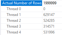
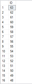
On my machine, the table takes less than 40 seconds to populate. We can see that the minimum and maximum IDs for each rowgroup are nice and neat from the sys.column_store_segments DMV:

a7_lucky

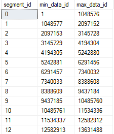
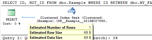
This table does not have any rowgroup elimination fragmentation. The segments are optimally constructed from a rowgroup elimination point of view. SQL Server will be able to skip every rowgroup except for one or two if I filter on a sequential range of one million integers:

SELECT COUNT(*)
FROM dbo.LUCKY_CCI
WHERE ID BETWEEN 12345678 AND 13345677;

STATISTICS IO output:

Table ‘LUCKY_CCI’. Segment reads 2, segment skipped 98.

Erik Darling was the inspiration for this next table, since he can never manage to get rowgroup elimination in his queries. The code below is designed to create segments that allow for pretty much no rowgroup elimination whatsoever:

DROP TABLE IF EXISTS dbo.UNLUCKY_CCI;

CREATE TABLE dbo.UNLUCKY_CCI (
	ID BIGINT NOT NULL,
	INDEX CCI CLUSTERED COLUMNSTORE
);

INSERT INTO dbo.UNLUCKY_CCI WITH (TABLOCK)
SELECT rg.RN
FROM
(
	SELECT TOP (100) ROW_NUMBER()
		OVER (ORDER BY (SELECT NULL)) RN
	FROM master..spt_values t1
) driver
CROSS APPLY (
	SELECT driver.RN

	UNION ALL

	SELECT 104857601 - driver.RN

	UNION ALL

	SELECT TOP (1048574) 100 + 1048574 * (driver.RN - 1)
		+ ROW_NUMBER() OVER (ORDER BY (SELECT NULL))
	FROM master..spt_values t2
	CROSS JOIN master..spt_values t3
) rg
ORDER BY driver.RN
OPTION (MAXDOP 1, NO_PERFORMANCE_SPOOL);

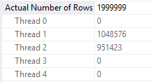
Each rowgroup will contain an ID near the minimum (1 – 100) and an ID near the maximum (104857301 – 104857400). We can see this with the same DMV as before:

a7_unlucky

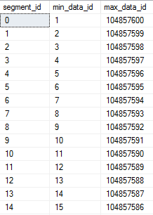
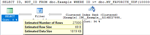
This table has pretty much the worst possible rowgroup elimination fragmentation. SQL Server will not be able to skip any rowgroups when querying almost any sequential range of integers:

SELECT COUNT(*)
FROM dbo.UNLUCKY_CCI
WHERE ID BETWEEN 12345678 AND 13345677;

STATISTICS IO output:

Table ‘UNLUCKY_CCI’. Segment reads 100, segment skipped 0.

Measuring Rowgroup Elimination Fragmentation

It might be useful to develop a more granular measurement for rowgroup elimination instead of just “best” and “worst”. One way to approach this problem is to define a batch size in rows for a filter against the column and to estimate how many total table scans would need to be done if the entire table was read in a series of SELECT queries with each processing a batch of rows. For example, with a batch size of 1048576 query, 1 would include the IDs from 1 to 1048576, query 2 would include IDs from 1 + 1048576 to 1048576 * 2, and so on. I will call this number the rowgroup elimination fragmentation factor, or REFF for short. It roughly represents how many extra rowgroups are read that could have been skipped with less fragmentation. Somewhat-tested code to calculate the REFF is below:

SET TRANSACTION ISOLATION LEVEL READ UNCOMMITTED;

DECLARE @batch_size INT = 1048576;
DECLARE @global_min_id BIGINT;
DECLARE @global_max_id BIGINT;
DECLARE @segments BIGINT;

DROP TABLE IF EXISTS #MIN_AND_MAX_IDS;
CREATE TABLE #MIN_AND_MAX_IDS (
	min_data_id BIGINT,
	max_data_id BIGINT
);
CREATE CLUSTERED INDEX c ON #MIN_AND_MAX_IDS
(min_data_id, max_data_id);

INSERT INTO #MIN_AND_MAX_IDS
SELECT css.min_data_id, css.max_data_id
FROM sys.objects o
INNER JOIN sys.columns c ON o.object_id = c.object_id
INNER JOIN sys.partitions p ON o.object_id = p.object_id
INNER JOIN sys.column_store_segments css
	ON p.hobt_id = css.hobt_id
	AND css.column_id = c.column_id
INNER JOIN sys.dm_db_column_store_row_group_physical_stats s
	ON o.object_id = s.object_id
	AND css.segment_id = s.row_group_id
	AND s.partition_number = p.partition_number
WHERE o.name = 'LUCKY_CCI'
AND c.name = 'ID'
AND s.[state] = 3;

SET @segments = @@ROWCOUNT;

SELECT
  @global_min_id = MIN(min_data_id)
, @global_max_id = MAX(max_data_id)
FROM #MIN_AND_MAX_IDS;

DROP TABLE IF EXISTS #BUCKET_RANGES;
CREATE TABLE #BUCKET_RANGES (
	min_data_id BIGINT,
	max_data_id BIGINT
);

 -- allows up to 6.4 million pieces
INSERT INTO #BUCKET_RANGES
SELECT
  @global_min_id + (RN - 1) * @batch_size
, @global_min_id + RN * @batch_size - 1
FROM
(
	SELECT ROW_NUMBER() OVER
	(ORDER BY (SELECT NULL)) RN
	FROM master..spt_values t1
	CROSS JOIN master..spt_values t2
) t
WHERE -- number of buckets
t.RN <= CEILING((1.0 * @global_max_id
	- (@global_min_id)) / @batch_size);

 -- number of total full scans
SELECT 1.0 * SUM(cnt) / @segments
FROM (
	SELECT COUNT(*) cnt
	FROM #BUCKET_RANGES br
	LEFT OUTER JOIN #MIN_AND_MAX_IDS m
		ON m.min_data_id <= br.max_data_id
 		AND m.max_data_id >= br.min_data_id
	GROUP BY br.min_data_id
) t;

For the LUCKY_CCI table, if we pick a batch size of 1048576 we get a REFF of 1.0. This is because each SELECT query would read exactly 1 rowgroup and skip the other 99 rowgroups. Conversely, the UNLUCKY_CCI table has a REFF of 100.0. This is because every SELECT query would need to read all 100 rowgroups just to return 1048576 rows. In other words, each query does a full scan of the table and there are 100 rowgroups in the table.

What about DUIs?

Suppose our lucky table runs out of luck and starts getting DUIs. As rows are deleted and reinserted they will be packed into new rowgroups. We aren’t likely to keep our perfect rowgroups for every long. Below is code that randomly deletes and inserts a range of 100k integers. There is some bias in which numbers are processed but that’s ok for this type of testing. I ran the code with 600 loops which means that up to 60% of the rows in the table could have been moved around. There’s nothing special about 60%. That just represents my patience with the process.

DECLARE @target_loops INT = 600,
@batch_size INT = 100001,
@current_loop INT = 1,
@middle_num BIGINT,
@rows_in_target BIGINT;

BEGIN

SET NOCOUNT ON;

SELECT @rows_in_target = COUNT(*)
FROM dbo.LUCKY_CCI;

DROP TABLE IF EXISTS #num;
CREATE TABLE #num (ID INT NOT NULL);

INSERT INTO #num WITH (TABLOCK)
SELECT TOP (@batch_size) -1 + ROW_NUMBER()
	OVER (ORDER BY (SELECT NULL)) RN
FROM master..spt_values t1
CROSS JOIN master..spt_values t2;

WHILE @current_loop <= @target_loops
BEGIN
	SET @middle_num = CEILING(@rows_in_target * RAND());

	DELETE tgt WITH (TABLOCK)
 	FROM dbo.LUCKY_CCI tgt
 	WHERE tgt.ID BETWEEN
 	CAST(@middle_num - FLOOR(0.5*@batch_size) AS BIGINT)
	AND
	CAST(@middle_num + FLOOR(0.5*@batch_size) AS BIGINT);

 	INSERT INTO dbo.LUCKY_CCI WITH (TABLOCK)
 	SELECT @middle_num + n.ID - FLOOR(0.5 * @batch_size)
	FROM #num n
 	WHERE n.ID BETWEEN 1 AND @rows_in_target
	OPTION (MAXDOP 1);

	SET @current_loop = @current_loop + 1;
END;

END;

Our table now has a bunch of uncompressed rowgroups and many compressed rowgroups with lots of deleted rows. Let’s clean it up with a REORG:

ALTER INDEX CCI ON dbo.LUCKY_CCI
REORGANIZE WITH (COMPRESS_ALL_ROW_GROUPS = ON);

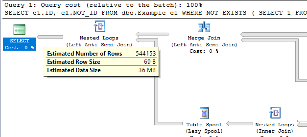
This table has a REFF of about 41 for a batch size of 1048576. That means that we can expect to see significantly worse rowgroup elimination than before. Running the same SELECT query as before:

Table ‘LUCKY_CCI’. Segment reads 51, segment skipped 75.

The LUCKY_CCI table clearly needs to be renamed.

The Magic of Partitioning

A partition for a CCI is a way of organizing rowgroups. Let’s create the same table but with partitions that can hold five million integers. Below is code to do that for those following along at home:

CREATE PARTITION FUNCTION functioning_part_function
(BIGINT)
AS RANGE RIGHT
FOR VALUES (
  0
, 5000000
, 10000000
, 15000000
, 20000000
, 25000000
, 30000000
, 35000000
, 40000000
, 45000000
, 50000000
, 55000000
, 60000000
, 65000000
, 70000000
, 75000000
, 80000000
, 85000000
, 90000000
, 95000000
, 100000000
, 105000000
); 

CREATE PARTITION SCHEME scheming_part_scheme
AS PARTITION functioning_part_function
ALL TO ( [PRIMARY] );

DROP TABLE IF EXISTS dbo.PART_CCI;

CREATE TABLE dbo.PART_CCI (
ID BIGINT NOT NULL,
INDEX CCI CLUSTERED COLUMNSTORE
) ON scheming_part_scheme(ID);

INSERT INTO dbo.PART_CCI WITH (TABLOCK)
SELECT TOP (100 * 1048576) ROW_NUMBER()
	OVER (ORDER BY (SELECT NULL)) RN
FROM master..spt_values t1
CROSS JOIN master..spt_values t2
CROSS JOIN master..spt_values t3
ORDER BY RN
OPTION (MAXDOP 1);

5 million was a somewhat arbitrary choice. The important thing is that it’s above 1048576 rows. Generally speaking, picking a partition size below 1048576 rows is a bad idea because the table’s rowgroups will never be able to reach the maximum size.

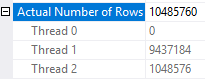
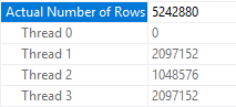
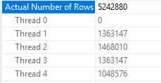
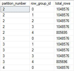
Using the sys.dm_db_column_store_row_group_physical_stats dmv we can see that rowgroups were divided among partitions as expected:

a7_part

This table has a REFF of 1.9 for a batch size of 1048576. This is perfectly reasonable because the partition size was defined as 5 * 1000000 instead of 5 * 1048576 which would be needed for a REFF of 1.0.

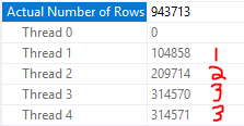
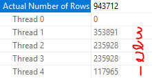
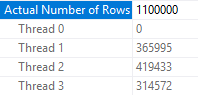
Now I’ll run the same code as before to do 60 million DUIs against the table. I expect the partitions to limit the damage because row cannot move out of their partitions. After the process finishes and we do a REORG, the table has a REFF of about 3.7. The rowgroups are definitely a bit messier:

a7_part_after_DUI

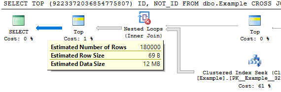
Running our SELECT query one last time:

SELECT COUNT(*)
FROM dbo.Part_CCI
WHERE ID BETWEEN 12345678 AND 13345677;

We see the following numbers for rowgroup elimination:

Table ‘PART_CCI’. Segment reads 4, segment skipped 3.

Only four segments are read. Many segments are skipped, including all of those in partitions not relevant to the query.

Final Thoughts

Large, unpartitioned CCIs will eventually run into issues with rowgroup elimination fragmentation if the loading process can delete data. A maintainance operation that rebuilds the table with a clustered rowstore index and rebuilds the CCI with MAXDOP = 1 is one way to restore nicely organized rowgroups, but that is a never-ending battle which grows more expensive as the table gets larger. Picking the right partitioning function can guarantee rowgroup elimination fragmentation. Thanks for reading!

Columnstore Parallel Scan Row Distribution

Parallel rowstore scans are parallel “aware”. This makes them unlike most other operators which work independently on different threads. Columnstore indexes store data in a dramatically different way than rowstore objects, so perhaps we can expect differences in how rows are distributed among threads during a parallel scan. This blog post explores some of the observable behavior around row distribution for parallel columnstore scans.

Methods of Rowstore Scan Parallel Row Distribution

This will be an extremely brief summary of how SQL Server distributes rows among threads for rowstore parallel scans. A parallel page supplier sends pages to each thread on a demand basis. Threads may end up processing different numbers of pages for many reasons. If you like, you can read more about this here and here. In addition, there is some fancy behavior for partitioned tables. The documentation describes this behavior in SQL Server 2008 and it may have changed since then, but this is sufficient to set the stage. The important part is that SQL Server will in some cases give each relevant partition its own thread. In other cases, SQL Server will assign multiple threads to a single partition.

Methods of Columnstore Scan Parallel Row Distribution

I investigated tables with only compressed rowgroups. I did not consider delta stores because real CCIs don’t have delta stores. As far as I can tell, there are at least three different methods that SQL Server can use to assign rows to threads during a parallel CCI scan.

Rowgroup Parallelism

One method of distributing rows is to assign each thread to a relevant rowgroup. Two or more threads will not read rows from the same rowgroup. This strategy can be used if the cardinality estimate from the scan is sufficiently high compared to the DOP used by the query. Rowgroup level parallelism will be used if:

Cardinality Estimate >= MAXDOP * 1048576 * 0.5

To show this, let’s build a CCI with a single column integer that runs from 1 to 1048576 * 10. Naturally, the table will have ten compressed rowgroups of the maximum size:

CREATE TABLE dbo.CCI_SHOW_RG_PARALLELISM (
	ID BIGINT NOT NULL,
	INDEX CCI CLUSTERED COLUMNSTORE
);

INSERT INTO dbo.CCI_SHOW_RG_PARALLELISM WITH (TABLOCK)
SELECT TOP (1048576 * 10) ROW_NUMBER()
	OVER (ORDER BY (SELECT NULL))
FROM master..spt_values t1
CROSS JOIN master..spt_values t2
CROSS JOIN master..spt_values t3
OPTION (MAXDOP 1);

I ran my tests with a simple query that is likely to go parallel on my machine and that doesn’t qualify for aggregate pushdown. With a cardinality estimate of exactly 1000000 and MAXDOP of 2 all of the rows are sent to one thread:

SELECT MAX(SQRT(ID))
FROM dbo.CCI_SHOW_RG_PARALLELISM
WHERE ID <= 1000000
OPTION (MAXDOP 2);

From the actual plan:

a6_RG_1

If we reduce the cardinality estimate by one row, the rows are spread out more evenly on the two threads:

SELECT MAX(SQRT(ID))
FROM dbo.CCI_SHOW_RG_PARALLELISM
WHERE ID <= 999999
OPTION (MAXDOP 2);

From the actual plan:

a6_RG_2

Note that the cardinality estimate displayed in SSMS may be misleading. The first query has a displayed cardinality estimate of 2000000 rows, but it does not use rowgroup parallelism:

SELECT MAX(SQRT(ID))
FROM dbo.CCI_SHOW_RG_PARALLELISM
WHERE ID <= 1999999 -- query plans can round
OPTION (MAXDOP 4);

From the actual plan:

a6_RG_3

But this one does:

SELECT MAX(SQRT(ID))
FROM dbo.CCI_SHOW_RG_PARALLELISM
WHERE ID <= 2000000
OPTION (MAXDOP 4);

From the actual plan:

a6_RG_4

Of course, we can get the query that takes an aggregate of 1999999 rows to use rowgroup level parallelism by bumping up the estimate:

DECLARE @filter BIGINT = 1999999;

SELECT MAX(SQRT(ID))
FROM dbo.CCI_SHOW_RG_PARALLELISM
WHERE ID <= @filter
OPTION (MAXDOP 4);

Here the estimate is:

0.3 * 10485800 = 3145740.0

So we get the expected parallelism strategy:

a6_RG_5

We can show that the rowgroup parallelism strategy is demand-based by deliberately slowing down the required the thread that grabs the first rowgroup in the table. Here I’m defining first by the ID that’s returned when running a SELECT TOP 1 ID query against the table. On my machine I get an ID of 9437185. The following code will add significant processing time in the CROSS APPLY part for only the row with an ID of 9437185. Every other row simply does a Constant Scan and goes on its merry way:

SELECT COUNT(*)
FROM dbo.CCI_SHOW_RG_PARALLELISM o
CROSS APPLY (
	SELECT TOP 1 1 c
	FROM
	(
		SELECT 1 c
		WHERE o.ID <> 9437185

		UNION ALL

		SELECT 1 c
		FROM master..spt_values t1
		CROSS JOIN master..spt_values t2
		CROSS JOIN master..spt_values t3
		WHERE o.ID = 9437185
		ORDER BY (SELECT NULL)
			OFFSET 100000000 ROWS
			FETCH FIRST 1 ROW ONLY
	) t
) t2
OPTION (MAXDOP 2);

Thread 1 processes nine rowgroups and waits on thread 2 to process its single rowgroup:

a6_RG_6

Split Rowgroup Parallelism

If the CCI has a small number of rows and the cardinality estimate is low enough you may see a different parallel row distribution strategy employed. I couldn’t think of a good name for this, but SQL Server splits up each rowgroup into roughly equal pieces and threads can process those pieces on a demand basis. The number of pieces seems to depend on the number of rows in the rowgroup instead of MAXDOP . For MAXDOP larger than 2 this behavior can be observed if a table has one or two rowgroups. For a MAXDOP of 2 this behavior can be observed if a table has exactly one rowgroup.

The formula for the number of pieces appears to be the number of rows in the rowgroup divided by 104857, rounded down, with a minimum of 1. The maximum rowgroup size of 1048576 implies a maximum number of pieces of 10 per rowgroup. Here’s a table to show all of the possibilities:

a6_table

We can see evidence of this behavior in SQL Server with a few tests. As before I’ll need to slow down one thread. First I’ll put 943713 integers into a single compressed rowgroup:

DROP TABLE IF EXISTS dbo.TEST_CCI_SMALL;

CREATE TABLE dbo.TEST_CCI_SMALL (
ID BIGINT NOT NULL,
INDEX CCI CLUSTERED COLUMNSTORE
);

INSERT INTO dbo.TEST_CCI_SMALL WITH (TABLOCK)
SELECT TOP (943713) ROW_NUMBER()
	OVER (ORDER BY (SELECT NULL))
FROM master..spt_values t1
CROSS JOIN master..spt_values t2
CROSS JOIN master..spt_values t3
OPTION (MAXDOP 1);

I will test with a very similar query to a previous test:

SELECT COUNT(*)
FROM dbo.TEST_CCI_SMALL o
CROSS APPLY (
	SELECT TOP 1 1 c
	FROM
	(
		SELECT 1 c
		WHERE o.ID <> 1

		UNION ALL

		SELECT 1 c
		FROM master..spt_values t1
		CROSS JOIN master..spt_values t2
		CROSS JOIN master..spt_values t3
		WHERE o.ID = 1
		ORDER BY (SELECT NULL)
			OFFSET 100000000 ROWS
			FETCH FIRST 1 ROW ONLY
	) t
) t2
OPTION (QUERYTRACEON 8649, MAXDOP 4);

The parallel scan should be split into nine pieces to be divided among threads because the table has a single rowgroup with a row count of 943713. This is exactly what happens:

a6_small_1

If I truncate the table and load one fewer row, the scan is now split up into eight pieces:

a6_small_2

I can also create two compressed rowgroups of a size that should led to seven pieces per rowgroup:

DROP TABLE IF EXISTS dbo.TEST_CCI_SMALL;

CREATE TABLE dbo.TEST_CCI_SMALL (
	ID BIGINT NOT NULL,
	INDEX CCI CLUSTERED COLUMNSTORE
);

INSERT INTO dbo.TEST_CCI_SMALL WITH (TABLOCK)
SELECT TOP (733999) ROW_NUMBER()
	OVER (ORDER BY (SELECT NULL))
FROM master..spt_values t1
CROSS JOIN master..spt_values t2
CROSS JOIN master..spt_values t3
OPTION (MAXDOP 1);

INSERT INTO dbo.TEST_CCI_SMALL WITH (TABLOCK)
SELECT TOP (733999) 733999 + ROW_NUMBER()
	OVER (ORDER BY (SELECT NULL))
FROM master..spt_values t1
CROSS JOIN master..spt_values t2
CROSS JOIN master..spt_values t3
OPTION (MAXDOP 1);

Thread 1 processes the row with an ID of 734000 so it only gets one piece:

a6_small_3

With more than one rowgroup, the demand-based aspect of piece distribution doesn’t quite work in the same way as with a single rowgroup. I wasn’t able to work out all of the details.

A Third Way?

What about queries that do not meet either of the two above criteria? For example, a query against a not small CCI that has a low cardinality estimate coming out of the scan? In some cases SQL Server will use rowgroup level distribution. In other cases it appears to use a combination of the two methods described above. Most of the time the behavior can be described as each thread gets assigned an entire rowgroup and threads race for pieces of the remaining rowgroups. I wasn’t able to figure out exactly how SQL Server decides which method to use, despite running many tests. However, I will show most of the behavior that I observed. First put 7 rowgroups into a CCI:

DROP TABLE IF EXISTS dbo.MYSTERIOUS_CCI;

CREATE TABLE dbo.MYSTERIOUS_CCI (
	ID BIGINT NOT NULL,
	INDEX CCI CLUSTERED COLUMNSTORE
);

INSERT INTO dbo.MYSTERIOUS_CCI WITH (TABLOCK)
SELECT TOP (1048576 * 7) ROW_NUMBER()
	OVER (ORDER BY (SELECT NULL))
FROM master..spt_values t1
CROSS JOIN master..spt_values t2
CROSS JOIN master..spt_values t3
OPTION (MAXDOP 1);

SELECT TOP 1 ID -- 6291457
FROM dbo.MYSTERIOUS_CCI;

I added local variables to my test query to lower the cardinality estimate. Otherwise I would get rowgroup distribution every time. Here’s an example query:

declare @lower_id INT = 1048576 * 2 + 1;
declare @upper_id INT = 1048576 * 7;

SELECT COUNT(*)
FROM dbo.MYSTERIOUS_CCI o
CROSS APPLY (
	SELECT TOP 1 1 c
	FROM
	(
		SELECT 1 c
		WHERE o.ID <> 6291457

		UNION ALL

		SELECT 1 c
		FROM master..spt_values t1
		CROSS JOIN master..spt_values t2
		CROSS JOIN master..spt_values t3
		WHERE o.ID = 6291457
		ORDER BY (SELECT NULL)
			OFFSET 100000000 ROWS
			FETCH FIRST 1 ROW ONLY
	) t
) t2
WHERE o.ID BETWEEN @lower_id AND @upper_id
OPTION (QUERYTRACEON 8649, MAXDOP 3);

With a MAXDOP of 3 and five processed rowgroups I get rowgroup level parallelism:

a6_3rd_1

With a MAXDOP of 4 and five processed rowgroups, each thread gets a rowgroup and the other three threads race to process the remaining 20 pieces:

a6_3rd_2

With a MAXDOP of 3 and six processed rowgroups we no longer get rowgroup level parallelism:

a6_3rd_3

What about Partitioning?

In tests not reproduced here, I was not able to observe any differences in how rows were distributed for parallel CCI scans when the underlying CCI was partitioned. This seems reasonable if we think about how partitioning for CCIs is different than for rowstore tables. CCI partitions are simply a collection of rowgroups containing rows relevant to the partition. If there’s a need to split up the underlying components of a table we can just assign rowgroups to different threads. For rowstore tables, we can think of each partition as a mini-table. Partitioning for rowstore adds underlying objects which can be distributed to parallel threads.

Fun with Query Plans

With a partial understanding of how SQL server distributes rows after a parallel scan, we can write queries that show some of the edge cases that can lead to poor performance. The following query is complete nonsense but it shows the point well enough. Here I’m cross joining to a few numbers from the spt_values table. The CROSS JOIN is meant to represent other downstream work done by a query:

SELECT MAX(SQRT(o.ID + t.number))
FROM dbo.MYSTERIOUS_CCI o
CROSS JOIN master..spt_values t
WHERE o.ID <= 1100000 AND
t.number BETWEEN 0 AND 4
OPTION (MAXDOP 2, NO_PERFORMANCE_SPOOL, QUERYTRACEON 8649);

The cardinality estimate and MAXDOP of 2 leads to rowgroup level parallelism being used. Unfortunately, this is very unbalanced:

a6_fun_1

And as a result, the query barely benefits from parallelism:

CPU time = 25578 ms, elapsed time = 24580 ms.

It’s a well-guarded secret that queries run faster with odd MAXDOP , so let’s try a MAXDOP of 3. Now my parallel threads no longer sleep on the job:

CPU time = 30922 ms, elapsed time = 11840 ms.

Here’s the row distribution from the scan:

a6_fun_2

Final Thoughts

This post explored a bit of the observable behavior for how rows are distributed to threads after a parallel columnstore index scan. The algorithms used can in some cases lead to row imbalance on threads which can cause performance issues downstream in the plan. The lack of repartition stream operators in batch mode can make this problem worse than it might be for rowstore scans, but I still expect issues caused by it to be relatively uncommon in practice. Thanks for reading!

Trace Flag 610 and SQL Server 2016

SQL Server recently surprised me with unexpected minimal logging. Normally this would be a cause for celebration but I was designing demos for a class. The point of that particular demo was to demonstrate a case in which minimal logging did not occur. The specific test case was inserting into a rowstore clustered index without a TABLOCK hint. Per the documentation, I should not have gotten minimal logging unless trace flag 610 was turned on. I was testing on SQL Server 2016 without trace flag 610.

Trace Flag 610

This trace flag is documented by Microsoft in The Data Loading Performance Guide. Here’s a relevant quote:

Not every row inserted in a cluster index with trace flag 610 is minimally logged. When the bulk load operation causes a new page to be allocated, all of the rows sequentially filling that new page are minimally logged. Rows inserted into pages that are allocated before the bulk load operation occurs are still fully logged, as are rows that are moved as a result of page splits during the load.

In addition, you can see a table of expected logging results if you search for “Summarizing Minimal Logging Conditions”. That table confirms that minimal logging should not happen when inserting into a clustered index without TABLOCK or trace flag 610. However, that’s exactly what I saw on SQL Server 2016.

SQL Server 2014 Testing

In a state of panic I immediately downloaded and installed SQL Server 2014 Express. Well not really, but it makes for a better blog post. For these tests I’m using a recovery model of simple.

Simple Inserts

First I’ll insert 2500 pages into a clustered rowstore table with a few different options. Table schema:

DROP TABLE IF EXISTS dbo.target_ci;

CREATE TABLE dbo.target_ci (
	ID BIGINT NOT NULL,
	FILLER VARCHAR(7700) NOT NULL,
	PRIMARY KEY (ID)
);

I’ll be checking out what’s getting logged with these queries:

SELECT SUM(database_transaction_log_bytes_used)
FROM sys.dm_tran_database_transactions
WHERE DATABASE_ID = 7;
-- you probably have a different database ID

SELECT Operation, COUNT(*)
FROM fn_dblog(NULL, NULL)
GROUP BY Operation
ORDER BY COUNT(*) DESC;

The first test is with TABLOCK, the second is without TABLOCK, and the third is without TABLOCK but with trace flag 610 enabled. I should get minimal logging for the first and the third and not for the second. Here’s the code that I ran:

CHECKPOINT;
BEGIN TRANSACTION;

INSERT INTO dbo.target_ci WITH (TABLOCK)
SELECT TOP (2500)
  ROW_NUMBER() OVER (ORDER BY (SELECT NULL))
, REPLICATE('Z', 7700)
FROM master..spt_values;

-- pause here

COMMIT TRANSACTION;
TRUNCATE TABLE dbo.target_ci;
CHECKPOINT;

BEGIN TRANSACTION;

INSERT INTO dbo.target_ci
SELECT TOP (2500)
  ROW_NUMBER() OVER (ORDER BY (SELECT NULL))
, REPLICATE('Z', 7700)
FROM master..spt_values;

-- pause here

COMMIT TRANSACTION;
TRUNCATE TABLE dbo.target_ci;
CHECKPOINT;

DBCC TRACEON(610);

BEGIN TRANSACTION;

INSERT INTO dbo.target_ci
SELECT TOP (2500)
  ROW_NUMBER() OVER (ORDER BY (SELECT NULL))
, REPLICATE('Z', 7700)
FROM master..spt_values;

-- pause here

COMMIT TRANSACTION;
TRUNCATE TABLE dbo.target_ci;
CHECKPOINT;

According the transaction log DMV, the first test logged 78,464 bytes, the second test logged 22,157,848 bytes, and the third logged 2,140,124 bytes. These results were expected. Below is a table of results from the undocumented fn_dblog TVF:

a5_2014_min_logging_table

I omitted out the (hopefully) irrelevant data. I don’t know what any of it means, but we can clearly see differences between the three tests. Based on this simple testing, SQL Server 2014 appears to match the documentation.

Page Splits

We can also do a simple test to show a case where trace flag 610 doesn’t help. First insert 2500 rows with odd primary keys from 1 to 4999:

CREATE TABLE dbo.NO_NEW_PAGES (
	ID BIGINT NOT NULL,
	DATA VARCHAR(3800),
	PRIMARY KEY (ID)
);

INSERT INTO dbo.NO_NEW_PAGES WITH (TABLOCK)
SELECT TOP (2500)
  -1 + 2 * ROW_NUMBER() OVER (ORDER BY (SELECT NULL))
, REPLICATE('Z', 3800)
FROM master..spt_values;

Then insert 2499 rows with even primary keys from 2 to 4998 with and without TF 610:

DBCC TRACEON(610);

BEGIN TRANSACTION;

INSERT INTO dbo.NO_NEW_PAGES
SELECT TOP (2499)
  2 * ROW_NUMBER() OVER (ORDER BY (SELECT NULL))
, REPLICATE('Z', 3800)
FROM master..spt_values;

-- pause here

ROLLBACK TRANSACTION;

DBCC TRACEOFF(610);

BEGIN TRANSACTION;

INSERT INTO dbo.NO_NEW_PAGES
SELECT TOP (2499)
  2 * ROW_NUMBER() OVER (ORDER BY (SELECT NULL))
, REPLICATE('Z', 3800)
FROM master..spt_values;

-- pause here

COMMIT TRANSACTION;

I expect a lot of page splitting because I can now fit two rows per page. TF 610 shouldn’t handle this scenario well. I logged 16,575,608 bytes with the trace flag and 9,796,224 bytes without the trace flag according to the transaction log DMV.

Nonclustered Indexes

Trace flag 610 can help with nonclustered indexes. Below is a test that inserts 2500 rows with and without trace flag 610 with an index on a new column:

CREATE TABLE dbo.IX_TEST (
	ID BIGINT NOT NULL,
	ID2 BIGINT NOT NULL,
	DATA VARCHAR(3800),
	PRIMARY KEY (ID)
);

CREATE INDEX IX ON IX_TEST (ID2);

DBCC TRACEON(610);

BEGIN TRANSACTION;

INSERT INTO dbo.IX_TEST
SELECT TOP (2500)
  ROW_NUMBER() OVER (ORDER BY (SELECT NULL))
, ROW_NUMBER() OVER (ORDER BY (SELECT NULL))
, REPLICATE('Z', 3800)
FROM master..spt_values;

-- pause here

ROLLBACK TRANSACTION;

DBCC TRACEOFF(610);

BEGIN TRANSACTION;

INSERT INTO dbo.IX_TEST
SELECT TOP (2500)
  ROW_NUMBER() OVER (ORDER BY (SELECT NULL))
, ROW_NUMBER() OVER (ORDER BY (SELECT NULL))
, REPLICATE('Z', 3800)
FROM master..spt_values;

-- pause here

COMMIT TRANSACTION;

There was an order of magnitude difference. With trace flag 610 I logged 1,129,728 bytes and without trace flag 610 I logged 10,120,144 bytes.

SQL Server 2016 Testing

I ran the same tests again on SQL Server 2016 SP1-CU3. With TABLOCK I logged 111,568 bytes according to the transaction log DMV. For both other tests I logged 2,125,376 bytes. Here’s a table of results from fn_dblog:

a5_2016_min_logging_table

Despite what the table says, note that the results with and without the trace flag weren’t exactly the same. However, even when running the same test sometimes the number of logged records per operation varies a little bit. My conclusion was that SQL Server is doing the same thing behind the scenes.

For both the page splitting and the nonclustered index test I got the same results as in SQL Server 2014. This shows that trace flag 610 does have some effect in SQL Server 2016, but not the one you’d expect from reading the documentation.

Estimated Final Thoughts

It appears that Microsoft has added additional minimal logging optimizations for clustered rowstore tables in SQL Server 2016. At least one of these optimizations was previously locked behind trace flag 610. I could not find any mention of this change in the documentation. If you carried over trace flag 610 when upgrading to SQL Server 2016, you should consider retesting that trace flag with your workload. It’s possible to construct a workload that benefits from trace flag 610 in SQL Server 2014 but is harmed by the same trace flag in SQL Server 2016.

Actual Final Thoughts

As of August 1, Microsoft documented that trace flag 610 is a no-op in SQL Server 2016. I revisited my results and found issues with the page splitting and nonclustered index tests. Starting with an empty table, inserting rows, and rolling back that transaction can affect the amount written to the log for future transactions. I don’t know why, but it’s necessary to drop and recreate the table before changing the trace flag to get clean results. It appears to be safe to turn off trace flag 610 in SQL Server 2016. Thanks for reading!

CCIs and String Aggregation

String aggregation is a not uncommon problem in SQL Server. By string aggregation I mean grouping related rows together and concatenating a string column for that group in a certain order into a single column. How will do CCIs do with this type of query?

The Data Set

A simple table with three columns is sufficient for testing. ITEM_ID is the id for the rows that should be aggregated together. LINE_ID stores the concatenation order within the group. COMMENT is the string column to be concatenated. The table will have 104857600 rows total with 16 rows per ITEM_ID.

CREATE TABLE dbo.CCI_FOR_STRING_AGG (
	ITEM_ID BIGINT NOT NULL,
	LINE_ID BIGINT NOT NULL,
	COMMENT VARCHAR(10) NULL,
	INDEX CCI CLUSTERED COLUMNSTORE
);

DECLARE @loop INT = 0
SET NOCOUNT ON;
WHILE @loop < 100
BEGIN
	INSERT INTO dbo.CCI_FOR_STRING_AGG WITH (TABLOCK)
	SELECT
	t.RN / 16
	, 1 + t.RN % 16
	, CHAR(65 + t.RN % 16)
	FROM
	(
		SELECT TOP (1048576)
		(1048576 * @loop) - 1 +
		ROW_NUMBER() OVER (ORDER BY (SELECT NULL)) RN
		FROM master..spt_values t1
		CROSS JOIN  master..spt_values t2
	) t
	OPTION (MAXDOP 1);

	SET @loop = @loop + 1;
END;

On my machine this codes takes around a minute and a half and the final table size is around 225 MB. I’m inserting batches of 1048576 rows with MAXDOP 1 to get nice, clean rowgroups.

The Test Query

Let’s concatenate the strings at an ITEM_ID level for all ITEM_IDs with an id between 3276800 and 3342335. All of the data is stored in a single rowgroup and the CCI was built in such a way that all other rowgroups can be skipped with that filter. This should represent the best case for CCI performance. A common way to concatenate a column is with the FOR XML PATH method:

SELECT
  o.ITEM_ID
, STUFF(
	(
		SELECT ','+ i.COMMENT
		FROM dbo.CCI_FOR_STRING_AGG i
		WHERE o.ITEM_ID = i.ITEM_ID
		ORDER BY i.LINE_ID
		FOR XML PATH('')
	)
,1 ,1, '') ALL_COMMENTS
FROM dbo.CCI_FOR_STRING_AGG o
WHERE o.ITEM_ID BETWEEN 3276800 AND 3342335
GROUP BY o.ITEM_ID;

Note that I’m not bothering with the additional arguments for the XML part, but you should whenever using this method in production.

The query plan looks reasonable at first glance:

a4 FOR XML estimated

However, the query takes nearly six minutes to complete. That’s not the lightning fast CCI query performance that we were promised!

Spool Problems

We can see from the actual execution plan that SQL Server scanned all 104.8 million rows from the CCI on a single thread:

a4 actual threads

Those rows were then sent into an index spool which was read from all four threads in the nested loop. The CCI scan and the build of the index spool took the most time in the plan so it makes sense why CPU time is less than elapsed time, even with a MAXDOP 4 query:

CPU time = 305126 ms, elapsed time = 359176 ms.

Thinking back to how parallel nested loop joins work, it seems unavoidable that the index spool was built with just one thread. The rows from the outer result set are sent to the inner query one row at a time on different threads. All of the threads run independently at MAXDOP 1. The eager spool for the index is a blocking operation and the blocking occurs even when the subquery isn’t needed. Consider the following query in which the ITEM_ID = 3400000 filter means that rows from the FOR XML PATH part of the APPLY will never be needed:

SELECT o.ITEM_ID
, ac.ALL_COMMENTS
FROM
(
	SELECT TOP (9223372036854775807) b.ITEM_ID
	FROM dbo.CCI_FOR_STRING_AGG b
	WHERE b.ITEM_ID BETWEEN 3276800 AND 3342335
	GROUP BY b.ITEM_ID
) o
OUTER APPLY (
	SELECT 'TEST'

	UNION ALL

	SELECT STUFF(
		(
			SELECT ','+ i.COMMENT
			FROM dbo.CCI_FOR_STRING_AGG i
			WHERE o.ITEM_ID = i.ITEM_ID
			ORDER BY i.LINE_ID
			FOR XML PATH('')
		)
	,1 ,1, '')
	WHERE o.ITEM_ID =  3400000
)  ac (ALL_COMMENTS)
OPTION (MAXDOP 4, QUERYTRACEON 8649);

The index spool is still built for this query on one thread even though the startup expression predicate condition is never met. It seems unlikely that we’ll be able to do anything about the fact that the index spool is built with one thread and that it blocks execution for the query. However, we know that we only need 1048576 rows from the CCI to return the query’s results. Right now the query takes 104.8 million rows and throws them into the spool. Can we reduce the number of rows put into the spool? The most obvious approach is to simply copy the filter on ITEM_ID into the subquery:

SELECT
  o.ITEM_ID
, STUFF(
	(
		SELECT ','+ i.COMMENT
		FROM dbo.CCI_FOR_STRING_AGG i
		WHERE o.ITEM_ID = i.ITEM_ID
		and i.ITEM_ID BETWEEN 3276800 AND 3342335
		ORDER BY i.LINE_ID
		FOR XML PATH('')
	)
,1 ,1, '') ALL_COMMENTS
FROM dbo.CCI_FOR_STRING_AGG o
WHERE o.ITEM_ID BETWEEN 3276800 AND 3342335
GROUP BY o.ITEM_ID;

This doesn’t have the desired effect:

a4 bad filter with spool

The filter is moved after the index build. We’ll still get all of the rows from the table put into the spool, but no rows will come out unless ITEM_ID is between 3276800 and 3342335. This is not helpful. We can get more strict with the query optimizer by adding a superfluous TOP to the subquery. That should force SQL Server to filter on ITEM_ID before sending rows to the spool because otherwise the TOP restriction may not be respected. One implementation:

SELECT
o.ITEM_ID
, STUFF(
(
SELECT ','+ i.COMMENT
FROM
(
SELECT TOP (9223372036854775807)
a.ITEM_ID, a.LINE_ID, a.COMMENT
FROM dbo.CCI_FOR_STRING_AGG a
WHERE a.ITEM_ID BETWEEN 3276800 AND 3342335
) i
WHERE o.ITEM_ID = i.ITEM_ID
ORDER BY i.LINE_ID
FOR XML PATH('')
)
,1 ,1, '') ALL_COMMENTS
FROM dbo.CCI_FOR_STRING_AGG o
WHERE o.ITEM_ID BETWEEN 3276800 AND 3342335
GROUP BY o.ITEM_ID;

SQL Server continues to outsmart us:

a4 no spool

As you can see in the plan above, the spool has completely disappeared. I was not able to find a way, even with undocumented black magic, to reduce the number of rows going into the spool. Perhaps it is a fundamental restriction regarding index spools. In fact, we can use the undocumented trace flag 8615 to see that spools are not even considered at any part in the query plan for the new query. On the left is the previous query with the spool with an example highlighted. On the right is the new query. The text shown here is just for illustration purposes, but we can see the spool on the left:

a4 TF diff

The important point is that for this query we appear to be stuck.

Rowgroup Elimination Problems

We can try our luck without the spool by relying on rowgroup elimation alone. The spool can’t be eliminated with the NO_PERFORMANCE_SPOOL hint, but another option (other than the TOP trick above) is to use the undocumented QUERYRULEOFF syntax to disable the optimizer rule for building spools:

SELECT
  o.ITEM_ID
, STUFF(
	(
		SELECT ','+ i.COMMENT
		FROM dbo.CCI_FOR_STRING_AGG i
		WHERE o.ITEM_ID = i.ITEM_ID
		ORDER BY i.LINE_ID
		FOR XML PATH('')
	)
,1 ,1, '') ALL_COMMENTS
FROM dbo.CCI_FOR_STRING_AGG o
WHERE o.ITEM_ID BETWEEN 3276800 AND 3342335
GROUP BY o.ITEM_ID
OPTION (QUERYRULEOFF BuildSpool);

The spool is gone but we don’t get rowgroup elimination:

a4 no RG elimination

We can get rowgroup elimination even without hardcoded filters with a bitmap from a hash join. Why don’t we get it with a nested loop join? Surely SQL Server ought to be able to apply rowgroup elimination for each outer row as it’s processed by the inner part of the nested loop join. We can explore this question further with tests that don’t do string aggregation. The query below gets rowgroup elimination but the constant filters are passed down to the CCI predicate:

SELECT *
FROM (VALUES (1), (2), (3), (4)) AS v(x)
INNER JOIN dbo.CCI_FOR_STRING_AGG a ON v.x = a.ITEM_ID
OPTION (FORCE ORDER, LOOP JOIN);

If we throw the four values into a temp table:

SELECT x INTO #t
FROM (VALUES (1), (2), (3), (4)) AS v(x)

The join predicate is applied in the nested loop operator. We don’t get any rowgroup elimination. Perhaps TOP can help us:

SELECT *
FROM #t v
CROSS APPLY (
	SELECT TOP (9223372036854775807) *
	FROM dbo.CCI_FOR_STRING_AGG a
	WHERE v.x = a.ITEM_ID
) a
OPTION (LOOP JOIN);

Sadly not:

a4 top failure

The join predicate is applied in the filter operation. We still don’t get any rowgroup elimination. Frustratingly, we get the behavior that we’re after if we replace the CCI with a heap:

a4 heap success

I don’t really see an advantage in pushing down the predicate with a heap. Perhaps Microsoft did not program the optimization that we’re looking for into the query optimizer. After all, this is likely to be a relatively uncommon case. This query is simple enough in that we filter directly against the CCI. In theory, we can give our query a fighting chance by adding a redundant filter on ITEM_ID to the subquery. Here’s the query that I’ll run:

SELECT
  o.ITEM_ID
, STUFF(
	(
		SELECT ','+ i.COMMENT
		FROM dbo.CCI_FOR_STRING_AGG i
		WHERE o.ITEM_ID = i.ITEM_ID
		and i.ITEM_ID BETWEEN 3276800 AND 3342335
		ORDER BY i.LINE_ID
		FOR XML PATH('')
	)
,1 ,1, '') ALL_COMMENTS
FROM dbo.CCI_FOR_STRING_AGG o
WHERE o.ITEM_ID BETWEEN 3276800 AND 3342335
GROUP BY o.ITEM_ID
OPTION (QUERYRULEOFF BuildSpool);

Unfortunately performance is even worse than before. The query finished in around 51 minutes on my machine. It was a proper parallel query and we skipped quite a few rowgroups:

Table ‘CCI_FOR_STRING_AGG’. Segment reads 65537, segment skipped 6488163.
CPU time = 10028282 ms, elapsed time = 3083875 ms.

Skipping trillions of rows is impressive but we still read over 68 billion rows from the CCI. That’s not going to be fast. We can’t improve performance further with this method since there aren’t any nonclustered indexes on the CCI, so there’s nothing better to seek against in the inner part of the loop.

Temp Tables

We can use the humble temp table to avoid some of the problems with the index spool. We’re able to insert into it in parallel, build the index in parallel, and we can limit the temp table to only the 1048576 rows that are needed for the query. The following code finishes in less than two seconds on my machine:

CREATE TABLE #CCI_FOR_STRING_AGG_SPOOL (
	ITEM_ID BIGINT NOT NULL,
	LINE_ID BIGINT NOT NULL,
	COMMENT VARCHAR(10) NULL
);

INSERT INTO #CCI_FOR_STRING_AGG_SPOOL WITH (TABLOCK)
SELECT a.ITEM_ID, a.LINE_ID, a.COMMENT
FROM dbo.CCI_FOR_STRING_AGG a
WHERE a.ITEM_ID BETWEEN 3276800 AND 3342335;

CREATE CLUSTERED INDEX CI_CCI_FOR_STRING_AGG_SPOOL
ON #CCI_FOR_STRING_AGG_SPOOL (ITEM_ID, LINE_ID);

SELECT
  o.ITEM_ID
, STUFF(
	(
		SELECT ','+ i.COMMENT
		FROM #CCI_FOR_STRING_AGG_SPOOL i
		WHERE o.ITEM_ID = i.ITEM_ID
		ORDER BY i.LINE_ID
		FOR XML PATH('')
	)
,1 ,1, '') ALL_COMMENTS
FROM dbo.CCI_FOR_STRING_AGG o
WHERE o.ITEM_ID BETWEEN 3276800 AND 3342335
GROUP BY o.ITEM_ID;

The query plan for the last query:

a4 temp table

With this approach we’re not really getting much from defining the underlying table as a CCI. If the table had more columns that weren’t needed then we could skip those columns with column elimination.

Other Solutions

An obvious solution is simply to add a covering nonclustered index to the table. Of course, that comes with the admission that columnstore currently doesn’t have anything to offer with this type of query. Other solutions which are likely to be more columnstore friendly include using a CLR function to do the aggregation and the SQL Server 2017 STRING_AGG function.

Note that recursion is not likely to be a good solution here. Every recursive query that I’ve seen involves nested loops. The dreaded index spool returns:

a4 recursion issue

Final Thoughts

Note that the poor performance of these queries isn’t a problem specific to columnstore. Rowstore tables can have the similar performance issues with string aggregation if there isn’t a sufficient covering index. However, if CCIs are used as a replacement for all nonclustered indexes, then the performance of queries that require the table to be on the inner side of a nested loop join may significantly degrade. Some of the optimizations that make querying CCIs fast appear to be difficult to realize for these types of queries. The same string aggregation query when run against a table with a rowstore clustered index on ITEM_ID and LINE_ID finished in 1 second. That is an almost 360X improvement over the CCI. Thanks for reading!

Returning All Rows with TABLESAMPLE

This post explores some undocumented behavior with TABLESAMPLE, specifically around the REPEATABLE option. TABLESAMPLE is a very useful tool to get a fast page-based sample of large tables. SQL Server uses it behind the scenes to gather sampled statistics.

Syntax

For this post we only need to be concerned with a subset of the syntax:

TABLESAMPLE SYSTEM (sample_number PERCENT )
[ REPEATABLE (repeat_seed) ]

Here’s a quote from that page about how TABLESAMPLE works internally:

TABLESAMPLE SYSTEM returns an approximate percentage of rows and generates a random value for each physical 8-KB page in the table. Based on the random value for a page and the percentage specified in the query, a page is either included in the sample or excluded.

One theory for how TABLESAMPLE works is that SQL Server generates a sequence of random values and does an allocation order scan that skips a page if the random value for that page does not meet the sample percent threshold. If REPEATABLE is used then SQL Server will generate the same sequence of random values each time, but results may be different if the table’s data has changed:

The REPEATABLE option causes a selected sample to be returned again. When REPEATABLE is specified with the same repeat_seed value, SQL Server returns the same subset of rows, as long as no changes have been made to the table. When REPEATABLE is specified with a different repeat_seed value, SQL Server will typically return a different sample of the rows in the table. The following actions to the table are considered changes: inserting, updating, deleting, index rebuilding, index defragmenting, restoring a database, and attaching a database.

How repeatable is REPEATABLE?

One might expect to get the same sample of pages with the REPEATABLE option even if the underlying data has changed but all of the pages remain in the same physical order. It also seems reasonable to think that if we add a page to the end of a table that the sample should stay the same except the new page may or may not be included in the sample. We can do some quick tests:

DROP TABLE IF EXISTS dbo.REPEATABLE_TEST;

CREATE TABLE dbo.REPEATABLE_TEST (
ID BIGINT NOT NULL IDENTITY(1, 1),
FILLER VARCHAR(7000),
PRIMARY KEY (ID)
);

INSERT INTO dbo.REPEATABLE_TEST
VALUES (REPLICATE('Z', 7000));
INSERT INTO dbo.REPEATABLE_TEST
VALUES (REPLICATE('Z', 7000));
INSERT INTO dbo.REPEATABLE_TEST
VALUES (REPLICATE('Z', 7000));
INSERT INTO dbo.REPEATABLE_TEST
VALUES (REPLICATE('Z', 7000));
INSERT INTO dbo.REPEATABLE_TEST
VALUES (REPLICATE('Z', 7000));
INSERT INTO dbo.REPEATABLE_TEST
VALUES (REPLICATE('Z', 3000));

-- returns 3 - 6
-- we skipped the first two pages 
-- and included the last four
SELECT ID
FROM dbo.REPEATABLE_TEST
TABLESAMPLE (50 PERCENT)
REPEATABLE (1);

INSERT INTO dbo.REPEATABLE_TEST
VALUES (REPLICATE('Z', 3000));

-- returns 3 - 7, same pages as before
SELECT ID
FROM dbo.REPEATABLE_TEST
TABLESAMPLE (50 PERCENT)
REPEATABLE (1);

INSERT INTO dbo.REPEATABLE_TEST
VALUES (REPLICATE('Z', 7000));

-- returns 3 - 8, includes new page
SELECT ID
FROM dbo.REPEATABLE_TEST
TABLESAMPLE (50 PERCENT)
REPEATABLE (1);

INSERT INTO dbo.REPEATABLE_TEST
VALUES (REPLICATE('Z', 7000));

-- returns 3 - 8, does not include new page
SELECT ID
FROM dbo.REPEATABLE_TEST
TABLESAMPLE (50 PERCENT)
REPEATABLE (1);

So far so good. However, the quote about REPEATABLE also calls out doing an index rebuild. We can see that our table isn’t fragmented at all with this query:

SELECT
  index_level
, page_count
, avg_fragmentation_in_percent
FROM sys.dm_db_index_physical_stats
(7, OBJECT_ID(N'dbo.REPEATABLE_TEST')
, NULL, NULL , 'DETAILED');

Result set:

a3_result_set_1

With a MAXDOP 1 rebuild I wouldn’t expect the physical order of pages to change at all. Indeed it doesn’t:

a3_result_set_1

We issue the REBUILD:

ALTER TABLE dbo.REPEATABLE_TEST REBUILD WITH (MAXDOP = 1);

However, now we get a completely different sample, despite the table still having no fragmentation. Pages 1, 2, 3, 5, and 8 are included in the results. The table has the same data and physical order as before. Why should the sample change even with the same REPEATABLE value?

Decoding REPEATABLE

Perhaps the REPEATABLE value is somehow combined with some piece of metadata with the table, similar to a salt used for encryption. The OBJECT_ID seems like a reasonable guess except that it won’t change after a rebuild. However, the HOBT_ID of the table does change after a REBUILD. We may be able to get a repeatable sample even after a REBUILD if we’re able to factor in the HOBT_ID somehow.

First let’s put 2537 pages into a new testing table:

DROP TABLE IF EXISTS dbo.REPEATABLE_SALT_TEST;

CREATE TABLE dbo.REPEATABLE_SALT_TEST (
ID BIGINT NOT NULL,
FILLER VARCHAR(7000),
PRIMARY KEY (ID)
);

INSERT INTO dbo.REPEATABLE_SALT_TEST WITH (TABLOCK)
SELECT
  ROW_NUMBER() OVER (ORDER BY (SELECT NULL))
, REPLICATE('Z', 7000)
FROM master..spt_values;

REPEATABLE allows between 1 and the maximum BIGINT value, 9223372036854775807. However, it’s easy to show through testing that a REPEATABLE value will return the same sample as REPEATABLE value + 4294967296. Perhaps picking a REPEATABLE value of hobt_id % 4294967296 will return the same sample even through a REBUILD.

SELECT hobt_id % 4294967296
FROM sys.partitions
where object_id = OBJECT_ID('REPEATABLE_SALT_TEST');

SELECT COUNT(*), MIN(ID), MAX(ID)
FROM dbo.REPEATABLE_SALT_TEST
TABLESAMPLE (50 PERCENT)
REPEATABLE (1248067584); -- use query value

I get 1306 pages sampled with a minimum value of 3 and a maximum value of 2537. After a REBUILD I get different results:

ALTER TABLE dbo.REPEATABLE_SALT_TEST
REBUILD WITH (MAXDOP = 1);

SELECT hobt_id % 4294967296
FROM sys.partitions
where object_id = OBJECT_ID('REPEATABLE_SALT_TEST');

SELECT COUNT(*), MIN(ID), MAX(ID)
FROM dbo.REPEATABLE_SALT_TEST
TABLESAMPLE (50 PERCENT)
REPEATABLE (1248133120); -- use query value

Now I get 1272 pages sampled with a minimum value of 6 and a maximum value of 2537. Through trial and error I arrived at one formula which works:

4294967296 - ((hobt_id + @salt) % 4294967296)

Where @salt is a positive integer between 1 and 4294967295. Let’s go back to our current testing table and use a @salt value of 1:

SELECT 4294967296 - ((hobt_id + 1) % 4294967296)
FROM sys.partitions
where object_id = OBJECT_ID('REPEATABLE_SALT_TEST');

SELECT COUNT(*), MIN(ID), MAX(ID)
FROM dbo.REPEATABLE_SALT_TEST
TABLESAMPLE (50 PERCENT)
REPEATABLE (3046768639);

Now I get 1268 pages sampled with a minimum value of 1 and a maximum value of 2534. After the rebuild I get the same result:

ALTER TABLE dbo.REPEATABLE_SALT_TEST
REBUILD WITH (MAXDOP = 1);

SELECT 4294967296 - ((hobt_id + 2147483648) % 4294967296)
FROM sys.partitions
where object_id = OBJECT_ID('REPEATABLE_SALT_TEST')

SELECT COUNT(*), MIN(ID), MAX(ID)
FROM dbo.REPEATABLE_SALT_TEST
TABLESAMPLE (50 PERCENT)
REPEATABLE (899219456); -- use query value

The formula can also be expressed as:

4294967296 - ((hobt_id + ABS(2147483648 - @salt)) % 4294967296)

With @salt as a positive integer from 0 to 2147483647. This is because there are repeated values in a cycle of 4294967296. More importantly, picking a @seed value of 1 always returns all pages from a table regardless of the sample size.

I admit that there is probably a simpler formula that I missed. Also, none of the above applies to columnstore tables. I doubt that it applies for partitioned rowstore tables as well but I did not test that.

Practical Applications?

There are a few interesting things that can be done with the new knowledge that we have around how REPEATABLE works.

Force an Allocation Order Scan

Normally you can only get an allocation order scan on a table with 64 pages or more unless you use TABLESAMPLE with a sample rate of less than 100%. However, now that we have a seed value that returns all rows no matter what we can force an allocation scan for any size table that returns all rows. Consider a 63 page table written to disk in the wrong order:

DROP TABLE IF EXISTS dbo.FORCE_ALLOCATION_ORDER_SCAN;

CREATE TABLE dbo.FORCE_ALLOCATION_ORDER_SCAN (
	ID BIGINT NOT NULL,
	PAGE_TURNER VARCHAR(5000) NOT NULL,
	PRIMARY KEY (ID)
);

-- add 63 pages with one row per page
-- in reverse clustered index order
DECLARE @i INTEGER = 63;
SET NOCOUNT ON;
WHILE @i > 0
BEGIN
	INSERT INTO dbo.FORCE_ALLOCATION_ORDER_SCAN
	WITH (TABLOCK)
	SELECT @i, REPLICATE('Z', 5000);

	SET @i = @i - 1;
END;

This table is very fragmented from the point of view of SQL Server:

a3_FORCE_ALLOCATION_ORDER_SCAN_frag

Now let’s find the REPEATABLE value which returns all rows:

-- returns 899088385
SELECT 4294967296 - ((hobt_id + ABS(2147483648 - 1)) % 4294967296)
FROM sys.partitions
where object_id = OBJECT_ID('SAMPLE_ALLOCATION_ORDER_TEST');

SELECT ID
FROM dbo.FORCE_ALLOCATION_ORDER_SCAN
TABLESAMPLE SYSTEM (99.99999 PERCENT )
REPEATABLE (899088385);

Here is a subset of the results:

a3_FORCE_ALLOCATION_ORDER_SCAN_results

Change Cardinality Estimates

With a repeatable value that returns 100% of the rows in the table we can change the percent to change the cardinality estimate from the table as long as we don’t exceed 99.99999 PERCENT or so.

The below query has a row estimate of 1 row:

SELECT ID
FROM dbo.FORCE_ALLOCATION_ORDER_SCAN
TABLESAMPLE SYSTEM (0 PERCENT)
REPEATABLE (899088385);

Query plan:

a3_1_row_estimate

And this query has an estimate of 63 rows:

SELECT ID
FROM dbo.FORCE_ALLOCATION_ORDER_SCAN
TABLESAMPLE SYSTEM (99.99999 PERCENT)
REPEATABLE (899088385);

Query plan:

a3_63_row_estimate

Of course, if the hobt_id for the table ever changes then the results from the query will change. TOP with an OPTIMIZE FOR hint is a good alternative, but TOP PERCENT has the overhead of an added table spool.

Consistent Samples

Suppose I want to create a demo that shows TABLESAMPLE missing all pages with a 50% sample rate against a 20 page table. If I find a REPEATABLE value that works against a table on my machine it likely won’t work for the reader because it will have a different hobt_id. First I need to find a REPEATABLE value that works for my table:

DROP TABLE IF EXISTS dbo.SAMPLE_NO_ROWS;

CREATE TABLE dbo.SAMPLE_NO_ROWS (
	PAGE_TURNER VARCHAR(5000) NOT NULL
);

INSERT INTO dbo.SAMPLE_NO_ROWS WITH (TABLOCK)
SELECT TOP 20 REPLICATE('Z', 5000)
FROM master..spt_values t1;

DECLARE @random_seed BIGINT = 0,
@target_num_rows INT = 0,
@found_rows INT,
@stop INT = 0,
@dynamic_sql NVARCHAR(1000);

BEGIN

SET NOCOUNT ON;

WHILE @stop = 0
BEGIN
	SET @random_seed = @random_seed + 1;

	SET @dynamic_sql = N'SELECT @sampled_row_count = COUNT(*)
	FROM dbo.SAMPLE_NO_ROWS
	TABLESAMPLE SYSTEM (50 PERCENT)
	REPEATABLE(' + CAST(@random_seed AS NVARCHAR(20)) + ')';

	EXECUTE sp_executesql @dynamic_sql, N'@sampled_row_count int OUTPUT', @sampled_row_count = @found_rows OUTPUT;

	IF @found_rows = @target_num_rows
	BEGIN
		SET @stop = 1
	END;
END;

SELECT @random_seed;

END;

After a lengthy search I got a REPEATABLE value of 823223 on my machine. The following query returns a count of 0 rows:

SELECT COUNT(*)
FROM dbo.SAMPLE_NO_ROWS
TABLESAMPLE SYSTEM (50 PERCENT)
REPEATABLE(823223);

With a hobt_id value of 72057595285143552 we can figure out the @salt value:

SELECT 4294967296 - ((hobt_id + 3046928457) % 4294967296)
FROM sys.partitions
where object_id = OBJECT_ID('SAMPLE_NO_ROWS');

Now I can reproduce the demo from scratch:

DROP TABLE IF EXISTS dbo.SAMPLE_NO_ROWS;

CREATE TABLE dbo.SAMPLE_NO_ROWS (
	PAGE_TURNER VARCHAR(5000) NOT NULL
);

INSERT INTO dbo.SAMPLE_NO_ROWS WITH (TABLOCK)
SELECT TOP 20 REPLICATE('Z', 5000)
FROM master..spt_values t1;

SELECT 4294967296 - ((hobt_id + 3046928457) % 4294967296)
FROM sys.partitions
where object_id = OBJECT_ID('SAMPLE_NO_ROWS');

-- count of 0
SELECT COUNT(*)
FROM dbo.SAMPLE_NO_ROWS
TABLESAMPLE SYSTEM (50 PERCENT)
REPEATABLE(4294545335); -- use query value

Query plan:

a3_demo_0_rows

Final Thoughts

Many of the things that I’ll blog about won’t be suitable for production use, but this should be considered especially unsuitable. Microsoft could change the undocumented behavior described here at any time. However, until it is changed it can be useful for demos or for further experimentation. Thanks for reading!

The Query Without an Efficient Join

Sometimes simple changes to a query can lead to dramatic changes in performance. I often find it helpful to dig into the details as much as I can whenever this happens.

Test Data

All that’s needed is a table with a clustered key defined on both columns. The first column will always have a value of 1 and the second column will increment for each row. We need two identical tables and may change the number of rows inserted into both of them for some tests. Below is SQL to follow along at home:

DROP TABLE IF EXISTS dbo.outer_tbl;
DROP TABLE IF EXISTS dbo.inner_tbl;

CREATE TABLE dbo.outer_tbl (
ID1 BIGINT NOT NULL,
ID2 BIGINT NOT NULL,
PRIMARY KEY (ID1, ID2)
);

CREATE TABLE dbo.inner_tbl (
ID1 BIGINT NOT NULL,
ID2 BIGINT NOT NULL,
PRIMARY KEY (ID1, ID2)
);

INSERT INTO dbo.outer_tbl WITH (TABLOCK)
SELECT TOP (20000)
  1
, ROW_NUMBER() OVER (ORDER BY (SELECT NULL))
FROM master..spt_values t1
CROSS JOIN master..spt_values t2;

INSERT INTO dbo.inner_tbl WITH (TABLOCK)
SELECT TOP (20000)
  1
, ROW_NUMBER() OVER (ORDER BY (SELECT NULL))
FROM master..spt_values t1
CROSS JOIN master..spt_values t2;

UPDATE STATISTICS dbo.outer_tbl
WITH FULLSCAN;
UPDATE STATISTICS dbo.inner_tbl
WITH FULLSCAN;

The Query

The following query will return one row from outer_tbl if there is at least one row in inner_tbl with a matching value for ID1 and ID2. For our initial data this query will return all 20000 rows. The query optimizer unsurprisingly picks a merge join and the query finishes with just 15 ms of CPU time:

SELECT *
FROM dbo.outer_tbl o
WHERE EXISTS (
	SELECT 1
	FROM dbo.inner_tbl i
	WHERE o.ID1 = i.ID1
	AND o.ID2 = i.ID2
);

Query plan:

a2 original query

Now let’s make a small change:

SELECT *
FROM dbo.outer_tbl o
WHERE EXISTS (
	SELECT 1
	FROM dbo.inner_tbl i
	WHERE o.ID1 = i.ID1
	AND o.ID2 IN (-1, i.ID2)
);

Query plan:

a2 adjusted query

Now the query will return one row from outer_tbl if ID1 = -1 and there is at least one row in inner_tbl with a matching value for ID1 or if there is at least one row in inner_tbl with a matching value for ID1 and ID2. The query optimizer gives me a hash join and the query finishes with 11360 ms of CPU time. If I force a loop join the query finishes with 10750 ms of CPU time. If I force a merge join the query finishes with 112062 ms of CPU time. What happened?

The Problem

The problem becomes easier to see if we change both of the tables to have just one column. We know that ID1 always equals 1 for both tables so we don’t need it in the query for this data set. Here’s the new set of tables:

DROP TABLE IF EXISTS dbo.outer_tbl_single;
DROP TABLE IF EXISTS dbo.inner_tbl_single;

CREATE TABLE dbo.outer_tbl_single (
ID2 BIGINT NOT NULL,
PRIMARY KEY (ID2)
);

CREATE TABLE dbo.inner_tbl_single (
ID2 BIGINT NOT NULL,
PRIMARY KEY (ID2)
);

INSERT INTO dbo.outer_tbl_single WITH (TABLOCK)
SELECT TOP (20000)
ROW_NUMBER() OVER (ORDER BY (SELECT NULL))
FROM master..spt_values t1
CROSS JOIN master..spt_values t2;

INSERT INTO dbo.inner_tbl_single WITH (TABLOCK)
SELECT TOP (20000)
ROW_NUMBER() OVER (ORDER BY (SELECT NULL))
FROM master..spt_values t1
CROSS JOIN master..spt_values t2;

UPDATE STATISTICS dbo.outer_tbl_single
WITH FULLSCAN;
UPDATE STATISTICS dbo.inner_tbl_single
WITH FULLSCAN;

If I try to force a hash join:

SELECT *
FROM dbo.outer_tbl_single o
WHERE EXISTS (
	SELECT 1
	FROM dbo.inner_tbl_single i
	WHERE o.ID2 IN (-1, i.ID2)
)
OPTION (MAXDOP 1, HASH JOIN);

I get an error:

Msg 8622, Level 16, State 1, Line 27
Query processor could not produce a query plan because of the hints defined in this query. Resubmit the query without specifying any hints and without using SET FORCEPLAN.

That makes sense. Hash join requires an equality condition and there isn’t one. Attempting to force a merge join throws the same error. A loop join is valid but there’s a scan on the inner side of the loop:

SELECT *
FROM dbo.outer_tbl_single o
WHERE EXISTS (
	SELECT 1
	FROM dbo.inner_tbl_single i
	WHERE o.ID2 IN (-1, i.ID2)
)
OPTION (MAXDOP 1, NO_PERFORMANCE_SPOOL);

Query plan:

a2 single column loop join

Note that we don’t need to read the 400 million (20000 * 20000) rows from the inner table. This is a semi join so the loop stops as soon as it finds a matching row. On average we should read (1 + 20000) / 2 rows from the inner table before finding a match so the query should need to read 20000 * (1 + 20000) / 2 = 200010000 rows from the inner table. This is indeed what happens:

a2 single column loop join actual

Hash Join Performance

Let’s go back to the initial slow query with two columns. Why is the query eligible for a hash join? Looking at the details of the hash join we can see that the hash probe is only on the ID1 column:

a2 hash probe

With this data set we end up with the worst possible case for a hash join. All of the rows from the build will hash to the same value and no rows from the probe will be eliminated. It’s still a semi join, so while we don’t know what the order of the hash table is we can still expect to need to (1 + 20000) / 2 entries of the hash table on average before finding the first match. This means that we’ll need to check 200010000 entries in the hash table just for this query. Since all of the work is happening in the hash join we should also expect quadratic performance for this query compared to the number of the rows in the table. If we change the number of rows in the table we see the quadratic relationship:

a2 hash rows in table vs time

For the table scans in the query we’re likely to do allocation order scans so the data may not be fed into the hash join in index order. However I just created the tables and data is returned in order in other queries, so I’m going to assume that data is fed into the join in order in this case. You may voice your objections to this assumption in the comments. Of course, the final output of the join may not be in order. We can monitor the progress of the query in a lightweight way using sys.dm_exec_query_profiles with trace flag 7412 enabled. I tested with 40k rows in each table to get a longer running join. The number of rows processed every quarter second was not constant:

a2 hash graph 40k

In fact, the query seemed to speed up as time went on. This was unexpected. Perhaps the hash table is built in such a way that the earliest rows for a hash value are at the end of the linked list and the last values processed are at the start? That would explain why the beginning of the query had the lowest number of rows processed per second and the number of rows processed per second increased over time. This is complete speculation on my part and is very likely to be wrong.

The costing for the hash join with the new CE is disappointing. All of the information is available in the statistics to suggest that we’ll get the worst case for the hash join but the total query cost is only 0.75 optimizer units. The legacy CE does better with a total query cost of 100.75 optimizer units but the hash join is still selected.

Merge Join Performance

For merge join the data is only sorted by ID1 for the join:

a2 merge join

The other part of the join involving the ID2 column is processed as a residual. This is also a many-to-many join. Craig Freedman has a good explanation of how many-to-many joins can lead to a lot of extra work in the join operator:

Merge join can also support many-to-many merge joins. In this case, we must keep a copy of each row from input 2 whenever we join two rows. This way, if we later find that we have a duplicate row from input 1, we can play back the saved rows. On the other hand, if we find that the next row from input 1 is not a duplicate, we can discard the saved rows. We save these rows in a worktable in tempdb. The amount of disk space we need depends on the number of duplicates in input 2.

We have the maximum number of duplicates per possible. It seems reasonable to expect very bad performance along with lots of tempdb activity. Since we’re reading the data in order we might expect to see the maximum rate of rows processed per second to be at the beginning and for the query to slow down as time goes on. As ID2 increases we need to read through more and more previous rows in tempdb. My intuition does not match reality at all in this case. There’s some silly bug with sys.dm_exec_query_profiles that needs to be worked around (merge join always reports 0 rows returned), but the rows processed per second was linear:

a2 merge join graph 1

The logical reads for the join is also linear and stabilizes to 49 reads per row returned with 10k rows in the base table.

a2 merge join graph 2

The number of logical reads per row returned stabilizes to 95 when there are 20k rows in the base table. This doesn’t appear to be a coincidence. Perhaps the data stored in tempdb is stored in a format that does not preserve the original ordering. We can look at the merge_actual_read_row_count column from the DMV for the merge join to see that the number of rows read per row processed from the inner table approaches the number of rows in the table. The ramp up happens very quickly. The measurements aren’t very precise, but for the 20k row test I saw that the merge join had processed 380000 rows after just reading 20 rows from the inner table. That would explain why the logical reads and runtime of the merge join grows quadratically with the number of rows in the table but the number of rows processed per second appears to be constant for a given table size.

For the merge join the query optimizer appears to be aware of the problem. Many-to-many joins seem to have quite a bit of a penalty from a costing perspective. With the new CE we get a total query cost of 421.072 optimizer units. The legacy CE gives a very similar cost.

Loop Join Performance

For the loop join we need to pay attention the clustered index seek in the inner part of the join:

a2 loop join operator

The -1 predicate causes trouble here as well. A filter condition will only be used as a seek predicate if it can be safely applied to every row. With the -1 check we don’t have anything to seek against for the inner table, so we only seek against ID1. As before, we should expect to read 200010000 rows from the seek. Our expectations are met:

a2 rows read

This is the first join which exposes the problem in a direct way in the XML for the actual plan which is nice. However, the performance will be quadratic with the number of rows in the table as with hash join and merge join. This is the first query that we have a shot at fixing. All that we need to do is to write the join in such a way that a seek can always be performed against the ID2 column in the inner table. The fact that the column cannot be NULL makes this possible. Consider the following query:

SELECT *
FROM dbo.outer_tbl o
WHERE EXISTS (
	SELECT 1
	FROM dbo.inner_tbl i
	WHERE o.ID1 = i.ID1
	AND i.ID2 BETWEEN (
	CASE
	WHEN o.ID2 = -1 THEN -9223372036854775808
	ELSE o.ID2
	END
	)
	AND CASE
	WHEN o.ID2 = -1 THEN 9223372036854775807
	ELSE o.ID2
	END
	)
) OPTION (MAXDOP 1, LOOP JOIN); 

Note that I’m only using BETWEEN to work around a wordpress bug.

When o.ID2 = -1 the code simplifies to the following:

 WHERE o.ID1 = i.ID1
AND i.ID2 BETWEEN -9223372036854775808
AND 9223372036854775807

When o.ID2 <> -1 the code simplifies to the following:

WHERE o.ID1 = i.ID1
AND i.ID2 BETWEEN o.ID2 AND o.ID2

In other words, can we use the bounds of the BIGINT to create a seek on ID2 that can always be done:

a2 good seek

The improved query returns the results with just 47 ms of CPU time. Only 20000 rows are read from the index seek which is the best possible result for our data set. The estimated cost of the query is dramatically reduced to 3.51182 for the new CE, but that isn’t enough for it to be naturally chosen over the much less efficient hash join. That is unfortunate. As you might have guessed the LOOP JOIN hint is not necessary when using the legacy CE.

Manual Rewrites

We can avoid the problem all together by changing the join condition to allow joins to work in a much more natural way. Splitting it up with a UNION finishes very quickly with our sample data set:

SELECT *
FROM dbo.outer_tbl o
WHERE EXISTS (
	SELECT 1
	FROM dbo.inner_tbl i
	WHERE o.ID1 = i.ID1
	AND o.ID2 = i.ID2
)

UNION

SELECT *
FROM dbo.outer_tbl o
WHERE o.ID2 = -1 AND EXISTS (
	SELECT 1
	FROM dbo.inner_tbl i
	WHERE o.ID1 = i.ID1
);

Query plan:

a2 union query

Splitting it into two semijoins does fine as well, although the hash match (aggregate) at the end is a bit more expensive for this data set than the hash match (union) employed by the other query:

SELECT *
FROM dbo.outer_tbl o
WHERE EXISTS (
	SELECT 1
	FROM dbo.inner_tbl i
	WHERE o.ID1 = i.ID1
	AND o.ID2 = -1
) OR EXISTS (
	SELECT 1
	FROM dbo.inner_tbl i
	WHERE o.ID1 = i.ID1
	AND o.ID2 = i.ID2
);

Query plan:

a2 OR query

Fully optimizing the above query is an interesting exercise but Paul White already covered the problem quite well here.

Final Thoughts

At first glance the following query is a little suspicious but the worst case performance scenario wasn’t immediately obvious (at least to me):

SELECT *
FROM dbo.outer_tbl o
WHERE EXISTS (
	SELECT 1
	FROM dbo.inner_tbl i
	WHERE o.ID1 = i.ID1
	AND o.ID2 IN (-1, i.ID2)
);

In fact, it will even perform well for some data sets. However, as the number of duplicate rows for a single ID grows we can end up with a triangular join. I found it interesting that all three join types scaled in the same way. Thanks for reading!

Manipulating Cardinality Estimates with Scalar UDFs

For this post I’m using the legacy cardinality estimator on SQL Server 2016 SP1.

The Problem

Scalar user defined functions are evil but sometimes necessary. The following scenario will sound a bit contrived but it’s based on a real world problem. Suppose that end users can filter the amount of data returned by a query by inputting values into a UDF that does some kind of translation. Below is a sample schema:

CREATE TABLE dbo.Example (
ID BIGINT NOT NULL,
NOT_ID VARCHAR(100) NOT NULL,
PRIMARY KEY (ID));

INSERT INTO dbo.Example WITH (TABLOCK)
(ID, NOT_ID)
SELECT TOP (1000000)
  ROW_NUMBER() OVER (ORDER BY (SELECT NULL))
, REPLICATE('Example', 14)
FROM master..spt_values t1
CROSS JOIN master..spt_values t2;

GO

CREATE FUNCTION dbo.MY_FAVORITE_UDF (@ID BIGINT)
RETURNS BIGINT AS
BEGIN
	RETURN @ID;
END;

Consider the following part of a much bigger query:

SELECT ID, NOT_ID
FROM dbo.Example
WHERE ID >= dbo.MY_FAVORITE_UDF(100000)
AND ID <= dbo.MY_FAVORITE_UDF(900000); 

For this demo it’s not important that the UDF do anything so I must made it return the input. To keep things simple I’m not going to follow best practices around writing the query to avoid executing the UDFs for each row in the table.  With the legacy cardinality estimator we get a cardinality estimate of 30% of the rows in the base table for each unknown equality condition. This means that a BETWEEN against two UDFs will give a cardinality estimate of 9%. The important point is that the cardinality estimate will not change as the inputs for the UDFs change, except for the trivial case in which the inputs are the same. This can easily be seen by varying the inputs and looking at the estimated execution plans:

SELECT ID, NOT_ID
FROM dbo.Example
WHERE ID >= dbo.MY_FAVORITE_UDF(100000)
AND ID <= dbo.MY_FAVORITE_UDF(900000);

Query plan:

blog picture 1

SELECT ID, NOT_ID
FROM dbo.Example
WHERE ID >= dbo.MY_FAVORITE_UDF(500000)
AND ID <= dbo.MY_FAVORITE_UDF(499999);

Query plan:

blog picture 2

SELECT ID, NOT_ID
FROM dbo.Example
WHERE ID BETWEEN dbo.MY_FAVORITE_UDF(1)
AND dbo.MY_FAVORITE_UDF(1);

Query plan:

blog-picture-3.png

The cardinality estimate (CE) of just that simple query doesn’t really matter. But it could matter very much if that query was part of a larger query with other joins. The 9% estimate may not serve us well depending on the rest of the query and what end users tend to input. We might know that the end users tend to pick large or small ranges. Even if we don’t know anything about the end users, certain queries may do better with larger or smaller cardinality estimates.

Decreasing the Cardinality Estimate

Let’s suppose that we do some testing and find that a cardinality estimate of lower than 9% is the best choice for typical end user inputs. There are a few techniques available to decrease the cardinality estimate by a fixed percentage.

Method 1

First option is to use TOP PERCENT along with an OPTIMIZE FOR hint. I’m not really a fan of TOP PERCENT. The implementation always spools unless it gets optimized out with TOP (100) percent. It would be nice if it didn’t spool. Anyway, perhaps getting a different cardinality estimate is worth the spool. Below is one method to get a cardinality estimate of 3% of the base table:

DECLARE @top_percent FLOAT = 100;

SELECT TOP (@top_percent) PERCENT ID, NOT_ID
FROM dbo.Example
WHERE ID >= dbo.MY_FAVORITE_UDF(100000)
AND ID <= dbo.MY_FAVORITE_UDF(900000)
OPTION (OPTIMIZE FOR (@top_percent = 33.33333333));

Query plan:

blog picture 4

The percent value is a float so we can go almost anywhere between 0 – 9% for the final estimate. However, if we have to use scalar UDFs in this fashion there’s a chance that we’re doing it to write platform agnostic code. The TOP trick here isn’t likely to work in other platforms.

Method 2

Suppose we add another inequality against a UDF that’s guaranteed not to change the results. 0.3^3 = 0.027 so we would expect an estimate of 2.7%. That is indeed what happens:

SELECT ID, NOT_ID
FROM dbo.Example
WHERE ID >= dbo.MY_FAVORITE_UDF(100000)
AND ID <= dbo.MY_FAVORITE_UDF(900000)

-- redundant filter to change CE
AND ID > dbo.MY_FAVORITE_UDF(100000) - 1;

Query plan:

blog picture 5
We can also mix things up with OR logic to make more adjustments. The query below has a fixed CE of 4.59%:

SELECT ID, NOT_ID
FROM dbo.Example
WHERE ID >= dbo.MY_FAVORITE_UDF(100000)
AND ID <= dbo.MY_FAVORITE_UDF(900000)
-- redundant filter to change CE
AND (ID > dbo.MY_FAVORITE_UDF(100000) - 1
OR ID > dbo.MY_FAVORITE_UDF(100000) - 2);

Query plan:

blog picture 6

It should be possible to mix and match to get something close to the CE that you want. I need to reiterate that as the code is written this will lead to additional UDF executions per row. You can also use techniques with fixed CE that don’t involve UDFs if you’re confident that Microsoft won’t change the guesses for them (which for the legacy cardinality estimator is probably a pretty safe assumption at this point).

Increasing the Cardinality Estimate

In some cases we will want a cardinality estimate above 9%.

Method 1

The TOP PERCENT trick won’t work here since TOP on its own can’t increase a cardinality estimate. We can use OR logic with UDFs to raise the estimate. Consider this filter condition:

ID >= dbo.MY_FAVORITE_UDF(100000)
OR ID >= dbo.MY_FAVORITE_UDF(900000) - 1

The first inequality gives an estimate of 30% and the second inequality gives an estimate of (100% – 30%) * 30% = 21%. In total we would get an estimate of 51%. If we apply that twice we should get an overall estimate of 0.51 * 0.51 = 26.01% . This is indeed what happens:

SELECT ID, NOT_ID
FROM dbo.Example
WHERE (ID >= dbo.MY_FAVORITE_UDF(1)
OR ID >= dbo.MY_FAVORITE_UDF(1) - 1)
AND (ID <= dbo.MY_FAVORITE_UDF(2)
OR ID <= dbo.MY_FAVORITE_UDF(2) + 1);

Query plan:

blog picture 7

By adding more UDFs to the OR clauses we can increase the cardinality estimate further.

Method 2

For another way to do it we can take advantage of the fact that an inequality filter against a UDF has the same cardinality as the negated condition. That means that this:

SELECT ID, NOT_ID
FROM dbo.Example

EXCEPT

SELECT ID, NOT_ID
FROM dbo.Example
WHERE -- negate original expression
ID < dbo.MY_FAVORITE_UDF(100000)
OR ID > dbo.MY_FAVORITE_UDF(900000);

Will return the same results as the original query but have a much higher cardinality estimate. Writing it in a better way, we see a cardinality estimate of ~54.4%:

SELECT e1.ID, e1.NOT_ID
FROM dbo.Example e1
WHERE NOT EXISTS (
	SELECT 1
	FROM dbo.Example e2
	WHERE e1.ID = e2.ID
	-- negate original expression
	AND e2.ID < dbo.MY_FAVORITE_UDF(100000)
	OR e2.ID > dbo.MY_FAVORITE_UDF(900000)
);

Query plan:

blog picture 8
This can be adjusted up and down by adding additional UDFs. It comes with the cost of an additional join so it’s hard to think of an advantage of doing it this way.

Method 3

For a third option we can use the MANY() table-valued function developed by Adam Machanic. This function can be used to increase the cardinality estimate of a point in a plan by a whole number. If we want a cardinality estimate of 18% from the UDF it’s as easy as the following:

SELECT TOP (9223372036854775807) ID, NOT_ID
FROM dbo.Example
CROSS JOIN dbo.Many(2)
WHERE ID BETWEEN dbo.MY_FAVORITE_UDF(100000)
AND dbo.MY_FAVORITE_UDF(900000);

Query plan:

blog picture 9

I added the superfluous TOP to prevent the MANY() reference from getting moved around in the plan. This method has the disadvantage that it may not be platform-agnostic.

Hopefully you never find yourself in a situation where you need to use tricks like this. Thanks for reading!